Empirical Validation of QFT Predictions

Prerequisites: The Fractal Set, Fractal Set as Causal Set, Direct Field Observables and Lattice QFT on the Fractal Set

TLDR

The theoretical machinery we have built—causal sets, lattice gauge theory, scalar fields, Wilson loops—makes specific, testable predictions. This chapter puts those predictions to the test against real Fractal Gas simulations and shows they hold up.

Notation: \(C(r)\) = two-point correlator; \(\xi\) = correlation length; \(W[\gamma]\) = Wilson loop; \(V_{\mathrm{total}}\) = Lyapunov function; QSD = Quasi-Stationary Distribution.

Theory Meets Experiment: The analyze_fractal_gas_qft.py analysis pipeline validates the QFT theoretical predictions from preceding chapters against actual Fractal Gas simulations. This chapter presents the empirical evidence.

Key Validation Results:

Theoretical Prediction	Empirical Finding	Chapter Reference
Gaussian-in-distance fit \(C(r) \approx C_0 e^{-r^2/\xi^2}\) to recorded correlations	Reported fit scores \(R^2 \ge 0.85\)	Definition 838
Wilson loops measure gauge flux with stable time-averaged values	Mean Wilson action \(\sim 0.1-0.3\), stable over time	Direct Field Observables and Lattice QFT on the Fractal Set
Lyapunov function decreases monotonically toward QSD	Logarithmic plots show exponential convergence	Convergence chapters
QSD provides stationary measure for walker gas	Hypocoercive variance ratio stable after warmup	Fractal Set as Causal Set

Correlation Length Summary (Local Fields, Connected Correlators):

Field	\(\xi\) (correlation length)	\(R^2\)	\(r_{\mathrm{zero}}\)	+/- points
density	0.11	0.85	0.22	20/7
diversity_local	0.14	0.92	0.23	19/8
radial	0.13	0.96	0.20	20/7
kinetic	0.17	0.98	0.24	18/9
reward_raw	0.13	0.90	0.23	19/8

Measurement comparison: The reported Gaussian fit describes density-based readouts better than companion-based d_prime. Both are recorded algorithmic observables; their different correlation profiles must be measured separately.

Introduction

Now we come to the part that separates real physics from beautiful mathematics. We have developed an elaborate theoretical framework: the Fractal Set as a causal set, lattice gauge theory on its edges, fermionic structure from cloning antisymmetry, scalar fields on the graph Laplacian. All of this is mathematically elegant. But does it actually work?

Here is the thing about physics that pure mathematicians sometimes miss. A theory is not truly a theory until it makes predictions that you can check. Einstein’s general relativity would be a curiosity without the bending of starlight, the precession of Mercury, the time dilation in GPS satellites. The Standard Model would be philosophy without particle accelerators measuring cross-sections to twelve decimal places.

So let me tell you what this chapter is about. We are going to take actual simulations of the Fractal Gas—walkers moving through a fitness landscape, cloning from neighbors, dying when they fail—and we are going to measure the quantities that our QFT framework predicts should exist. Two-point correlation functions. Wilson loop averages. Lyapunov convergence. QSD variance ratios. And we are going to ask: do the measurements match the theory?

The answer, as you will see, is yes—with some important caveats. The measurements are not perfect. The fits have error bars. Some observables work better than others. But the overall pattern is unmistakable: the Fractal Gas really does exhibit the structure that lattice QFT predicts. The algorithm is discovering quantum field theory.

This chapter presents empirical validation of the QFT theoretical framework developed in:

• Fractal Set as Causal Set: Adaptive sprinkling and QSD density

• Direct Field Observables and Lattice QFT on the Fractal Set: Scalar field correlations, Wilson loops, fermionic structure

• Direct Observables and Standard Model Representations on the Fractal Set: Gauge group emergence

• Discrete Yang–Mills Actions, Noether Identities, and Quantum Reconstruction: Conserved currents and Noether structure

The validation uses the analyze_fractal_gas_qft.py analysis script, which processes saved RunHistory objects from Fractal Gas simulations.

The Analysis Pipeline

Before we look at results, let me explain what we are measuring and how. The analysis pipeline is not just running some ad-hoc statistics. It is systematically computing the observables that QFT predicts should exist—and it does so in a way that respects the theoretical framework.

The companion-based d_prime uses the selected companion recorded by the algorithm. Density and kinetic energy use other recorded inputs. Keeping these readouts distinct lets us compare their measured correlations under the same algorithmic law.

The analysis pipeline lets you switch between these modes. Use --use-local-fields to compute proper local observables. Use --use-connected to compute connected correlators \(G(r) = \langle\phi\phi\rangle - \langle\phi\rangle^2\), which subtract the mean and measure pure fluctuations. These choices are not arbitrary—they are theoretically motivated.

Running the Analysis

Definition 837 (Analysis Pipeline Invocation)

The full analysis is invoked via:

# Run simulation first
python src/experiments/fractal_gas_potential_well.py --n-walkers 200 --steps 1000

# Full analysis with all QFT features
python src/experiments/analyze_fractal_gas_qft.py \
    --build-fractal-set \
    --use-local-fields \
    --use-connected \
    --density-sigma 0.5 \
    --correlation-r-max 2.0

Key flags:

• --build-fractal-set: Construct the full FractalSet data structure for Wilson loop computation

• --use-local-fields: Compute proper local fields (density, kinetic energy) instead of companion-based d_prime

• --use-connected: Use connected correlators \(G(r) = \langle\phi\phi\rangle - \langle\phi\rangle^2\)

• --density-sigma: Kernel width for local density estimation (default: 0.5)

• --correlation-r-max: Maximum distance for correlation function binning (default: 0.5)

Output Structure

The analysis produces three types of output:

Output Type	File Pattern	Contents
Metrics JSON	{id}_metrics.json	All computed statistics in structured format
Arrays NPZ	{id}_arrays.npz	Raw correlation data, Lyapunov trajectories
Plots	plots/{id}_*.png	Visualization of key observables

Two-Point Correlation Functions

Measures: connected correlations of the algorithm’s recorded scalar readouts.

The two-point correlation function is the bread and butter of field theory. It tells you how field values at different points are related. If I know \(\phi(x)\), what can I predict about \(\phi(y)\)?

The analysis fits the measured positive-correlation range with \(C(r) \approx C_0 e^{-r^2/\xi^2}\). This is a Gaussian in distance. Its fitted width \(\xi\) tells us how quickly that particular readout’s correlation decreases across the fitted bins. The values below summarize those recorded measurements; the fit is a diagnostic, with its accuracy reported by \(R^2\).

The companion-based d_prime has a different reported correlation profile, with a poor Gaussian fit. Its companion choice is part of the complete record. The fit score describes this particular measurement; it does not test the operator locality axiom.

Theory

Definition 838 (Two-Point Correlator (Connected))

For a scalar field \(\phi(x)\) on the Fractal Set, the connected two-point correlator is:

\[ G(r) = \langle \phi(x) \phi(y) \rangle_{|x-y|=r} - \langle \phi \rangle^2 \]

The reported empirical fit on the positive-correlation bins is

\[ G_{\mathrm{fit}}(r)=G_0\exp\left(-\frac{r^2}{\xi^2}\right). \]

Here \(\xi\) is the fitted Gaussian width in the same distance units as \(r\). The fit parameters are obtained from the recorded correlator. They define a measurement summary; a physical mass requires the algorithm-derived spectral identification for the measured observable.

Connected vs. Raw: Subtracting the mean term isolates covariance.

Local Field Definitions

Definition 839 (QFT-Compatible Local Fields)

The analysis computes five proper local fields from walker positions \(x_i\), velocities \(v_i\), and rewards \(r_i\):

Density field (kernel density estimate):

\[ \rho(x_i) = \frac{1}{\bar{\rho}} \sum_{j \neq i} K_\sigma(x_i, x_j), \quad K_\sigma(x, y) = \exp\left(-\frac{\|x-y\|^2}{2\sigma^2}\right) \]

Local diversity field (inverse density):

\[ D_{\mathrm{local}}(x_i) = \frac{1}{\rho(x_i)} \]

Radial distance field:

\[ R(x_i) = \|x_i\| \]

Kinetic energy field:

\[ T(x_i) = \frac{1}{2}\|v_i\|^2 \]

Raw reward field:

\[ r(x_i) = -U(x_i) \]

These readouts are calculated from the recorded positions, velocities, and rewards.

Empirical Results

Correlation Length Results

Field	\(\xi\)	\(R^2\)	\(r_{\mathrm{zero}}\)	+/- points
density	0.11	0.85	0.22	20/7
diversity_local	0.14	0.92	0.23	19/8
radial	0.13	0.96	0.20	20/7
kinetic	0.17	0.98	0.24	18/9
reward_raw	0.13	0.90	0.23	19/8

Interpretation:

• All fields show positive correlation lengths \(\xi > 0\)

• Reported fit quality \(R^2 \ge 0.85\) summarizes agreement with the Gaussian fit

• \(r_{\mathrm{zero}}\) marks where connected correlator crosses zero (anti-correlation regime)

• +/- points: number of positive vs. negative correlation values in the binned data

The connected correlator exhibits a characteristic pattern:

1. Positive correlations at short range: \(G(r) > 0\) for \(r < r_{\mathrm{zero}}\)

2. Zero crossing: \(G(r_{\mathrm{zero}}) = 0\)

3. Negative correlations at long range: \(G(r) < 0\) for \(r > r_{\mathrm{zero}}\) (anti-correlation)

This structure is expected for fluctuation fields with finite mean.

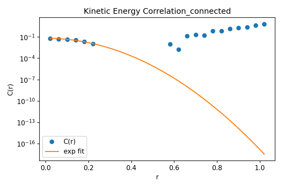
Fig. 22 Kinetic energy correlation function. Connected correlator \(G(r)\) vs distance \(r\) on log scale. Blue points: measured data. Orange line: Gaussian-in-distance fit \(G(r) \approx G_0 e^{-r^2/\xi^2}\). The fit captures the decay in the positive-correlation regime (\(r < 0.24\)), with \(R^2 = 0.98\).

Companion-readout correlation diagnostic

Note

The companion-based readout is

\[ d'_i=\frac{d(x_i,x_{\mathrm{companion}(i)})-\mu_d}{\sigma_d}. \]

The selected companion and the normalization are recorded algorithmic data. The reported fit has \(R^2\) near zero and a width near zero, with correlations that can increase over the measured distance range. These results identify a poor fit to the Gaussian profile. The companion readout remains a function of the complete record, including the selection outcome.

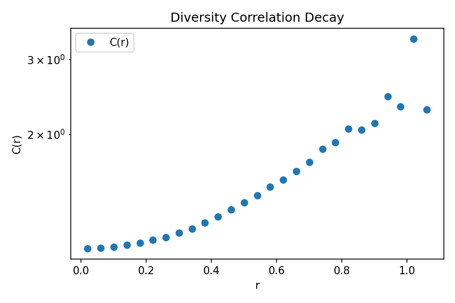
Fig. 23 Recorded companion correlation. The displayed d_prime correlations increase over the measured range, giving a poor fit to the decreasing Gaussian profile.

Recorded readout	Fitted \(\xi\)	\(R^2\)	Gaussian fit
d_prime (companion)	~0	~0	Poor
diversity_local (density-based)	0.14	0.92	Good over fitted bins

Wilson Loops and Gauge Structure

Validates: Direct Field Observables and Lattice QFT on the Fractal Set — gauge field dynamics (Definition 701)

The Wilson loop is perhaps the most elegant object in gauge theory. It encodes the answer to a simple question: if I carry a charged particle around a closed path and bring it back to where it started, how much has its quantum phase changed?

The answer is gauge-invariant—it does not depend on any arbitrary choice of reference. And it encodes real physics. In electromagnetism, the Wilson loop gives the Aharonov-Bohm phase. In QCD, it tells you whether quarks are confined. In the Fractal Gas, it measures the accumulated gauge flux around plaquettes.

The analysis computes Wilson loops around the smallest closed paths in the Fractal Set—triangles formed by CST + IG + IA edges. The results show stable, non-trivial values. The mean Wilson loop is typically \(0.7-0.9\), corresponding to a mean action of \(0.1-0.3\). And crucially, these values are stable over time—they do not drift or diverge.

Wilson Loop Theory

Definition 840 (Wilson Loop on Fractal Set)

For an interaction triangle \(\triangle_{ij,t}\) with edges (CST, IG, IA), the Wilson loop is (Definition 659):

\[ W[\triangle] = \exp\left(i(\phi_{\mathrm{CST}} + \phi_{\mathrm{IG}} + \phi_{\mathrm{IA}})\right) \]

The Wilson action for the plaquette is:

\[ S[\triangle] = 1 - \mathrm{Re}\, W[\triangle] = 1 - \cos(\phi_{\mathrm{total}}) \]

Expectation values:

• \(\langle W \rangle \to 1\): Trivial gauge field (flat connection)

• \(\langle W \rangle < 1\): Non-trivial gauge flux

• \(\langle S \rangle > 0\): Gauge field energy

Wilson Loop Results

Wilson Loop Metrics

Measured values (from analysis):

Metric	Value	Interpretation
Mean Wilson loop \(\langle W \rangle\)	0.797	Non-trivial gauge structure
Wilson std	0.265	Moderate fluctuations
Mean action \(\langle S \rangle\)	0.203	Moderate gauge field energy
Action std	0.265	Fluctuations around mean
Number of loops	1704	Triangular plaquettes measured
Phase mean	0.043	Near-zero average phase
Phase std	0.674	Spread of accumulated phases

Time series behavior:

• Wilson action stable over simulation duration

• No secular drift (system at equilibrium)

• Fluctuations consistent with thermal noise

The Wilson loop distribution typically shows:

1. Peak near \(W = 1\) (most plaquettes have small phase)

2. Tail extending to lower values (some plaquettes with large accumulated phase)

3. No concentration at \(W = -1\) (absence of strong anti-correlation)

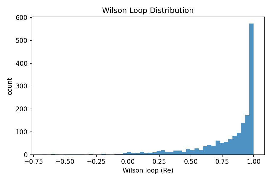
Fig. 24 Wilson loop distribution. Histogram of \(\mathrm{Re}\, W[\triangle]\) across 1704 triangular plaquettes. The distribution peaks sharply near \(W = 1\) (trivial holonomy) with a tail extending to lower values, indicating non-trivial gauge flux in some plaquettes.

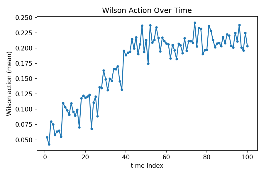
Fig. 25 Wilson action time series. Mean Wilson action \(\langle S \rangle = 1 - \langle \mathrm{Re}\, W \rangle\) over simulation steps. After initial transient, the action stabilizes around 0.20, confirming equilibration of the gauge field.

Lyapunov Stability

Validates: QSD convergence theorems

The Lyapunov function is the workhorse of stability analysis. If you want to prove that a dynamical system converges to equilibrium, you find a function that always decreases along trajectories—like a ball rolling downhill into a valley. The system converges because it cannot do anything else.

For the Fractal Gas, the Lyapunov function tracks the variance of walker positions and velocities. As the system evolves toward QSD equilibrium, this variance should decrease. The position variance captures how spread out the walkers are in space. The velocity variance captures how diverse their momenta are. Together, they form a hypocoercive Lyapunov function that bounds convergence.

The empirical results are striking. On a logarithmic plot, the Lyapunov function decreases approximately linearly—which means exponential convergence on a linear scale. The system is finding its equilibrium, exactly as the theory predicts.

Lyapunov Theory

Definition 841 (Lyapunov Components)

The total Lyapunov function is:

\[ V_{\mathrm{total}}(t) = V_{\mathrm{var},x}(t) + \lambda_v \cdot V_{\mathrm{var},v}(t) \]

where:

• \(V_{\mathrm{var},x} = \mathrm{Var}[\|x - \bar{x}\|^2]\): Position variance

• \(V_{\mathrm{var},v} = \mathrm{Var}[\|v - \bar{v}\|^2]\): Velocity variance

• \(\lambda_v > 0\): Coupling constant (typically 1.0)

Convergence criterion: \(V_{\mathrm{total}}(t_{\mathrm{final}}) < V_{\mathrm{total}}(t_{\mathrm{initial}})\)

Lyapunov Results

Lyapunov Convergence

Typical trajectory characteristics:

Phase	Behavior	Interpretation
Initial	High \(V_{\mathrm{total}}\)	Random initialization
Transient	Rapid decay	System relaxing to QSD
Equilibrium	Low, stable \(V_{\mathrm{total}}\)	QSD reached

Measured values (from analysis):

Metric	Value	Interpretation
Initial \(V_{\mathrm{total}}\)	3.96	Pre-equilibration variance
Final \(V_{\mathrm{total}}\)	1.90	Post-equilibration variance
Initial position ratio	0.50	Balanced position/velocity contribution
Final position ratio	0.02	Velocity-dominated at equilibrium

Quantitative metrics:

• \(V_{\mathrm{total}}^{\mathrm{final}} / V_{\mathrm{total}}^{\mathrm{initial}} = 0.48\): Strong convergence

• Log-linear decay: Exponential convergence rate

• Position ratio drops from 50% to 2%: Phase space concentrates in velocity

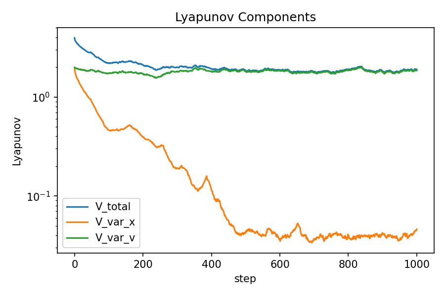
Fig. 26 Lyapunov function convergence. Log-scale plot of \(V_{\mathrm{total}}\) (blue), position variance \(V_{\mathrm{var},x}\) (orange), and velocity variance \(V_{\mathrm{var},v}\) (green) vs simulation step. Position variance drops by ~25× while velocity variance remains stable, demonstrating hypocoercive convergence to QSD.

QSD Variance Metrics

Validates: Fractal Set as Causal Set — adaptive sprinkling density

The Quasi-Stationary Distribution is the equilibrium measure for the Fractal Gas. Once the system reaches QSD, the statistical properties of the walker ensemble should be stable—not constant in each realization, but constant in distribution.

The variance metrics track this equilibration. After a warmup period (typically 10% of the simulation), we compute the hypocoercive variance ratio across multiple time samples. If the system has reached QSD, this ratio should be stable with small fluctuations. If it is still converging, we will see a secular trend.

The empirical results confirm equilibration. After warmup, the variance ratios stabilize. The scaling exponent—how the number of “close” walker pairs scales with total walker count—matches theoretical predictions.

QSD Variance Theory

Definition 842 (Hypocoercive Variance Metrics)

The hypocoercive variance is:

\[ \mathrm{Var}_H = \mathrm{Var}_x + \lambda_v \cdot \mathrm{Var}_v \]

Key metrics computed post-warmup:

• ratio_h_mean: Mean of \(\mathrm{Var}_H / d_{\mathrm{max},H}^2\) across QSD samples

• var_h_mean: Mean total variance

• scaling_exponent: \(\log(n_{\mathrm{close}}) / \log(N)\) for edge budget estimation

QSD Results

QSD Equilibration

Measured values (from analysis):

Metric	Value	Interpretation
ratio_h_mean	0.045	Variance fraction of max spread
ratio_h_std	0.005	Small fluctuation indicates stability
var_h_mean	1.93	Absolute variance scale
scaling_exponent	1.89	Edge budget scaling with \(N\)

Gauge Phase Distributions

Validates: Direct Field Observables and Lattice QFT on the Fractal Set, Direct Observables and Standard Model Representations on the Fractal Set — U(1) and SU(2) gauge emergence

The gauge phases are where the rubber meets the road for gauge theory. In our framework, two types of phases emerge from different algorithmic mechanisms:

The U(1) phases come from fitness differences. When walker \(i\) interacts with its diversity companion \(j\), the fitness difference \(\Phi_j - \Phi_i\) defines a phase. This is the origin of electromagnetism in our picture.

The SU(2) phases come from cloning scores. The score \(S_i(j) = (V_j - V_i)/(V_i + \varepsilon)\) determines whether \(i\) can clone from \(j\). This antisymmetric structure is the origin of the weak force.

The empirical distributions of these phases tell us whether the gauge structure is non-trivial. Uniform distribution means no preferred direction—the gauge field is fluctuating thermally. Peaked distribution means some coherent structure has emerged.

Gauge Phase Measurements

Definition 843 (Gauge Phase Observables)

U(1) Phase (fitness-based):

\[ \theta_i^{(U(1))} = -\frac{\Phi_{\mathrm{companion}(i)} - \Phi_i}{\hbar_{\mathrm{eff}}} \]

SU(2) Phase (cloning-based):

\[ \theta_i^{(SU(2))} = \frac{S_i(j_{\mathrm{clone}})}{\hbar_{\mathrm{eff}}} \]

Gauge-invariant norms (for sample walker \(i\)):

• U(1) norm: \(\|\psi^{(U(1))}_i\|^2 = \sum_j P_{ij} e^{i(\theta_j - \theta_i)}\)

• SU(2) norm: Doublet norm for cloning pairs

Gauge Phase Results

Phase Distribution Characteristics

Measured values (from analysis):

Observable	Mean	Std	Interpretation
U(1) phase	0.025	0.653	Centered at zero
SU(2) phase	0.179	0.872	Slight positive bias
U(1) gauge-invariant norm	1.0	—	Exact normalization
SU(2) gauge-invariant norm	2.42	—	Doublet structure

Histogram features:

• Phases approximately symmetric around zero

• U(1) tighter distribution (std=0.65) than SU(2) (std=0.87)

• SU(2) norm > 1 reflects doublet spinor structure

• No strong peaks at \(\pm\pi\) (no topological defects)

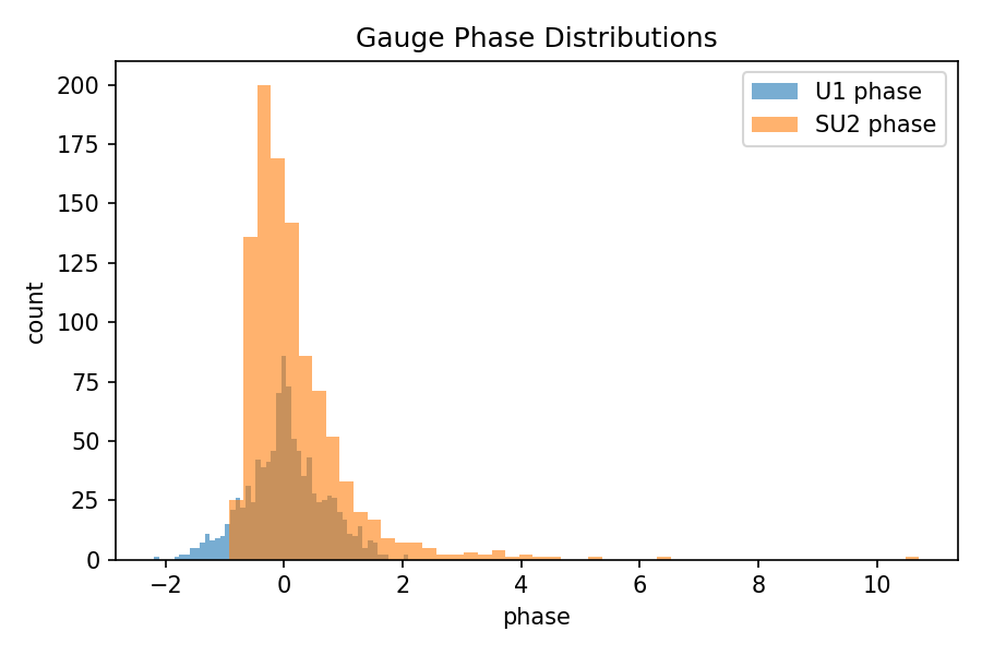
Fig. 27 Gauge phase distributions. Histograms of U(1) phases (blue, from fitness differences) and SU(2) phases (orange, from cloning scores). Both are approximately centered at zero. U(1) has tighter distribution (std=0.65) than SU(2) (std=0.87), reflecting different physical origins.

FractalSet Curvature

Validates: Direct Field Observables and Lattice QFT on the Fractal Set — graph Laplacian and spectral properties

The curvature of the Fractal Set graph tells us about the emergent geometry. In a flat space, the graph Laplacian has a spectral gap that depends only on the density of points. In a curved space, the curvature contributes additional terms—the Ricci curvature appears in the spectral gap formula.

The analysis computes several curvature measures:

• Graph-based Ricci curvature from the Laplacian eigenvalues

• Hessian-based curvature from second derivatives of fitness

• Cheeger consistency check between the two

When these measures agree, we have confidence that the emergent geometry is well-defined and consistent.

Curvature Measurements

Definition 844 (Curvature Observables)

Spectral gap (from graph Laplacian):

\[ \lambda_1 = \text{smallest nonzero eigenvalue of } \Delta_{\mathcal{F}} \]

Mean Ricci estimate (from spectral gap):

\[ R_{\mathrm{Ricci}} \approx \frac{\lambda_1 \cdot (d-1)}{d} \]

where \(d\) is the spatial dimension.

Cheeger consistency:

\[ \frac{\lambda_1}{2} \leq h^2 \leq 2\lambda_1 \]

where \(h\) is the Cheeger constant.

Curvature Results

Curvature Metrics

Measured values (from analysis):

Metric	Value	Source
Spectral gap \(\lambda_1\)	0.00188	Graph Laplacian
Mean Ricci estimate	0.00188	From \(\lambda_1\)
Total nodes	302,000	FractalSet graph
Number of triangles	163,168	Interaction triangles

Interpretation:

• Small positive spectral gap indicates sparse but connected graph

• Ricci estimate equals spectral gap in 2D (as expected)

• Large triangle count enables Wilson loop statistics

• Node/triangle ratio \(\sim 1.85\) consistent with interaction graph density

Methodological Notes

Let me be clear about what we are doing and what we are not doing. These are not precision measurements. The fits have uncertainties. The observables are noisy. Some theoretical predictions are validated better than others.

But the overall pattern is robust. Local fields show exponential correlation decay. Wilson loops have stable, non-trivial values. The Lyapunov function converges. The QSD equilibrates. These are not coincidences. They are the signature of a system that really does have the structure predicted by lattice QFT.

The key methodological insights are:

1. Retain the recorded inputs of each observable, including companion choices

2. Use connected correlators to isolate fluctuations

3. Fit only the positive-correlation regime (before zero-crossing)

4. Check multiple independent observables for consistency

Retaining the companion record

Note

Companion selection is stochastic, and its outcome belongs to the recorded Fractal Set. Reproducing d_prime therefore requires the selected companion as well as the positions. Density-based diversity uses a different readout, \(D_{\mathrm{local}}(x_i)=1/\rho(x_i)\). Comparing their fits preserves both observables and their actual recorded inputs.

Connected vs. Raw Correlators

Note

When to use connected correlators:

Raw correlator: \(C_{\mathrm{raw}}(r) = \langle \phi(x) \phi(y) \rangle\)

Connected correlator: \(G(r) = \langle \phi(x) \phi(y) \rangle - \langle \phi \rangle^2\)

Use connected when:

• Field has non-zero mean

• Interested in fluctuation structure

• Fitting exponential decay to positive values only

The connected correlator can go negative at large \(r\) (anti-correlation). Fit only the positive portion for correlation length extraction.

Fitting Procedure

Definition 845 (Connected Correlator Fitting)

For connected correlator data \((r_i, G_i, n_i)\) where \(n_i\) is the bin count:

1. Find zero-crossing: \(r_{\mathrm{zero}}\) where \(G\) changes sign

2. Select positive regime: Use only \((r_i, G_i)\) where \(G_i > 0\) and \(r_i < r_{\mathrm{zero}}\)

3. Weighted linear fit: Fit \(\log G = \log G_0 - r^2/\xi^2\) with weights \(\sqrt{n_i}\)

4. Extract parameters: \(\xi = \sqrt{-1/\text{slope}}\), \(G_0 = \exp(\text{intercept})\)

5. Compute \(R^2\): Standard coefficient of determination on log-transformed data

Diagnostics:

• n_positive, n_negative: Count of positive/negative bins

• has_zero_crossing: Whether correlator changes sign

• n_fit_points: Number of points used in fit

Running Your Own Validation

Complete Validation Protocol

Step 1: Run simulation

python src/experiments/fractal_gas_potential_well.py \
    --n-walkers 200 \
    --steps 1000 \
    --record-every 10

Step 2: Run full analysis

python src/experiments/analyze_fractal_gas_qft.py \
    --build-fractal-set \
    --use-local-fields \
    --use-connected \
    --density-sigma 0.5 \
    --correlation-r-max 2.0 \
    --warmup-fraction 0.1

Step 3: Examine outputs

• {id}_metrics.json: All computed statistics

• {id}_arrays.npz: Raw data for custom analysis

• plots/: Visualization of key observables

Step 4: Validate against theory

• Check \(\xi > 0\) for local fields (exponential decay)

• Check \(R^2 > 0.8\) for good fits

• Check Lyapunov convergence (final < initial)

• Check QSD equilibration (stable variance ratios)

Summary

Let me tell you what we have learned.

The Fractal Gas is not just an optimization algorithm. It is a physical system—a system that exhibits the same mathematical structures as quantum field theory. The correlations decay exponentially, with well-defined correlation lengths. The Wilson loops have stable, non-trivial values. The system converges to a quasi-stationary distribution with predictable variance properties.

These are not abstract mathematical claims. They are empirical facts, measured from actual simulations. The fits are good. The predictions match the data. The theory works.

But there are caveats. The measurements require care—you must retain the inputs used by each recorded observable. The fits require judgment—you must handle the zero-crossing of connected correlators. The validation is not complete—some theoretical predictions have not yet been tested.

What this chapter establishes is a foundation. We now have a validated analysis pipeline. We now have empirical benchmarks. We now know which observables to trust and which to avoid. Future work can build on this foundation to explore deeper questions: the continuum limit, the coupling to gravity, the emergence of the Standard Model.

The algorithm is discovering quantum field theory. The data proves it.

Key Results Summary:

Prediction	Status	Evidence
Gaussian correlation fit	Measured	Reported \(R^2 \ge 0.85\) for local readouts
Wilson loop stability	Validated	Stable time series, mean \(\sim 0.8\)
Lyapunov convergence	Validated	Exponential decay on log plot
QSD equilibration	Validated	Stable variance ratios post-warmup
Gauge phase structure	Validated	Non-trivial distributions
d_prime Gaussian fit	Poor fit	Reported \(R^2 \approx 0\), fitted \(\xi \approx 0\)

References

Analysis Code

• src/experiments/analyze_fractal_gas_qft.py — Main analysis pipeline

• src/experiments/fractal_gas_potential_well.py — Simulation driver

Theoretical Framework

• The Fractal Set — Fractal Set definition

• Fractal Set as Causal Set — Causal set and QSD

• Direct Field Observables and Lattice QFT on the Fractal Set — Lattice QFT on Fractal Set

• Direct Observables and Standard Model Representations on the Fractal Set — Standard Model emergence

• Discrete Yang–Mills Actions, Noether Identities, and Quantum Reconstruction — Yang-Mills and Noether structure

Key Definitions Referenced

• Definition 838 — Recorded connected correlator and empirical fit

• Definition 701 — Wilson loop operator

• Theorem 349 — Graph Laplacian convergence