
The Fractal Set#
TLDR#
Execution Record: The Fractal Set \(\mathcal{F} = (\mathcal{N}, E_{\mathrm{CST}} \cup E_{\mathrm{IG}} \cup E_{\mathrm{IA}}, \mathcal{T})\) is a 2-dimensional simplicial complex with an oriented 1-skeleton (a directed 2-complex) that organizes the declared recorded samples of the Fractal Gas algorithm’s execution. Nodes represent spacetime points (walker \(i\) at timestep \(t\)), CST edges encode temporal evolution, IG edges encode spatial coupling, and IA (influence attribution) edges close the causal loop from effect back to cause. The interaction triangles \(\mathcal{T}\) are the fundamental 2-simplices—each triangle records one complete interaction: “walker \(j\) influenced walker \(i\)’s evolution from \(t\) to \(t+1\).”
Covariant Storage: Nodes store scalar attributes. Edges and boundary records store directional payloads with declared Clifford, frame, and chart conventions. The equivariant decoder recovers correspondingly rotated vectors when these conventions are transformed consistently.
Directed Selection and Operator Reconstruction: IG edges record the signed fitness difference \(V_{\mathrm{clone}}(i \to j)=\Phi_j-\Phi_i\). The field chapters construct edge bilinears and the exact exterior-sector correspondence with independent process replicas; this specifies the operator meaning beyond the score’s sign reversal.
Triangular Interactions and Wilson Loops: The fundamental closed loops are 3-cycles (interaction triangles), not 4-cycles. Each triangle \(\triangle_{ij,t}\) has vertices \((n_{j,t}, n_{i,t}, n_{i,t+1})\) connected by IG, CST, and IA edges. Plaquettes (4-cycles) are derived structures: two adjacent triangles sharing a diagonal. Assigned edge transports define triangle holonomies. A plaquette holonomy is the ordered product of the triangle holonomies transported to a common basepoint; its trace is gauge invariant. For scalar \(U(1)\) transports, this reduces to ordinary multiplication of triangle phases.
Lossless Reconstruction Guarantee: A complete record includes initial and isolated-state anchors, the declared transition and cloning stages, terminal field evaluations when sampled, and tensor decoding conventions. It recovers the stored states, force and diffusion samples, scalar evaluations, empirical measures, and recorded noise increments. The identities are exact in real arithmetic; floating-point errors depend on precision and conditioning. Unrecorded intermediate timesteps are outside this guarantee.
Introduction#
A velocity is a geometric arrow; its stored components are numbers in a chosen frame. Rotating the frame changes those numbers, while preserving scalar measurements such as its norm. A spinor representation gives another way to encode the arrow, together with a precise rule for changing frames.
Keep the distinction between the geometric object and its serialization in mind. Reading spinor components requires the Clifford matrices, frame, chart, and encoding convention. Once these are supplied, the decoder is equivariant: rotating the encoded object rotates the recovered vector. This is what allows two observers to compare their reconstructions.
The Fractal Set organizes a declared execution record into scalar node data, covariant edge payloads, and the boundary and reference records needed to decode them. Its completeness statement concerns those recorded samples. The continuum analysis later uses the regularity and fluctuation estimates already established elsewhere in Volume 2.
The Fractal Gas algorithm generates a complex web of interacting walkers evolving through a state space, with dynamics governed by kinetic forces, fitness-dependent selection, and stochastic diffusion. A complete record of this algorithm’s execution must capture not only where each walker was at each timestep, but also the forces that acted upon it, the selection pressures it experienced, and the coupling with other walkers that influenced its cloning decisions.
The Fractal Set is designed to store all of this information with two key properties:
Frame covariance: A recorded frame and codec convention lets observers transform decoded components consistently and recover the same invariant observables.
Lossless completeness: The complete record includes its header and boundary payloads. Its decoder recovers every declared recorded sample by the explicit inverse identities below.
The structure separates data into two categories based on transformation properties:
Category |
Stored On |
Transformation |
Examples |
|---|---|---|---|
Scalars |
Nodes |
Invariant (same in all frames) |
Energy, fitness, status flags, norms |
Spinors |
Edges |
Covariant (transform under \(\mathrm{Spin}(d)\)) |
Velocities, forces, gradients, displacements |
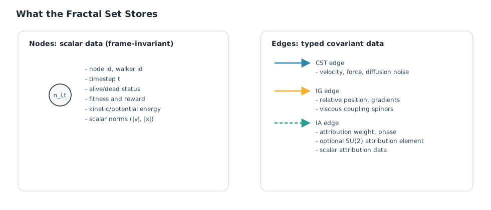
Fig. 15 What gets stored where. Nodes carry only scalar data; CST and IG edges carry spinor-encoded vectors; IA edges store scalar attribution weights and phases and, for non-abelian gauge, an SU(2) attribution element.#
The edges divide into three types reflecting the algorithm’s causal structure:
Edge Type |
Connects |
Encodes |
Directionality |
|---|---|---|---|
CST (Causal Spacetime Tree) |
\((n_{i,t}, n_{i,t+1})\) |
Temporal evolution of single walker |
Directed (time’s arrow) |
IG (Information Graph) |
\((n_{i,t}, n_{j,t})\) |
Spatial coupling between contemporaneous walkers |
Directed (selection asymmetry) |
IA (Influence Attribution) |
\((n_{i,t+1}, n_{j,t})\) |
Causal attribution from effect to cause |
Directed (retrocausal) |
Together, the three edge types form a directed 1-skeleton: CST encodes timelike evolution, IG encodes spacelike coupling, and IA closes causal triangles by attributing each walker’s update to its influencers. The underlying undirected support is simplicial.
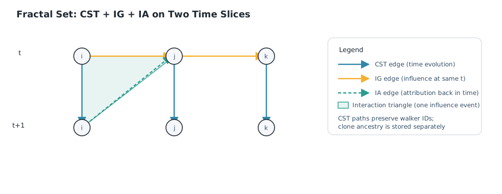
Fig. 16 Fractal Set on two time slices. CST edges run forward in time, IG edges connect same-time walkers, and IA edges point back from effects to causes. One interaction triangle is highlighted.#
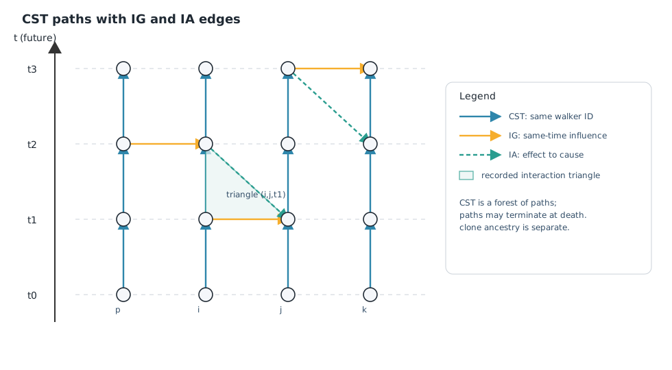
Fig. 17 CST paths with IG and IA edges. CST edges follow persistent walker IDs forward in time, while IG edges link contemporaneous walkers in sampled directed pairs and IA edges attribute influence back across timesteps. Clone ancestry is separate from the CST paths.#
Overview#
The Fractal Set captures the Fractal Gas algorithm as a 2-dimensional directed 2-complex with the following components:
Let \(\mathcal{P}_t\) denote the set of ordered companion pairs realized at timestep \(t\) by the companion selection operators (distance and cloning; Definition 663). Define \(m_t := |\mathcal{P}_t|\).
Nodes \(\mathcal{N}\) (0-simplices): One node \(n_{i,t}\) for each walker \(i \in \{1, \ldots, N\}\) at each timestep \(t \in \{0, 1, \ldots, T\}\). Total: \(|\mathcal{N}| = N(T+1)\) nodes.
CST Edges \(E_{\mathrm{CST}}\) (1-simplices): Directed edges \((n_{i,t}, n_{i,t+1})\) connecting consecutive timesteps of the same walker, provided the walker is alive at time \(t\). These form a forest of directed paths (one per persistent walker ID); genealogical links from cloning are recorded separately.
IG Edges \(E_{\mathrm{IG}}\) (1-simplices): Directed edges \((n_{i,t}, n_{j,t})\) for each sampled companion pair \((i, j) \in \mathcal{P}_t\) at the same timestep. At timestep \(t\) with \(k_t\) alive walkers, there are \(m_t\) directed IG edges (one per sampled ordered pair).
IA Edges \(E_{\mathrm{IA}}\) (1-simplices): Directed edges \((n_{i,t+1}, n_{j,t})\) connecting the effect (walker \(i\) at \(t+1\)) to the cause (walker \(j\) at \(t\)) for each \((i, j) \in \mathcal{P}_t\) with \(t \in \{0,\ldots,T-1\}\). These close the causal triangles, attributing each walker’s evolution to its sampled influencers. There are \(m_t\) IA edges per update timestep.
Clone ancestry graph \(E_{\mathrm{clone}}\) (derived): A directed relation from parent to child defined by the clone source attribute; these edges encode branching history but are not part of the CST order (see Definition 641).
Interaction Triangles \(\mathcal{T}\) (2-simplices): Each triangle \(\triangle_{ij,t}\) has vertices \(\{n_{j,t}, n_{i,t}, n_{i,t+1}\}\) and boundary edges (IG, CST, IA), for each \((i, j) \in \mathcal{P}_t\) and \(t \in \{0,\ldots,T-1\}\). These are the fundamental closed loops of the structure.
Weight functions: \(\omega_{\mathrm{CST}}: E_{\mathrm{CST}} \to \mathbb{R}_{>0}\) assigns temporal weights (typically \(\Delta t\)), \(\omega_{\mathrm{IG}}: E_{\mathrm{IG}} \to \mathbb{R}\) assigns selection coupling weights (the antisymmetric cloning potential), and \(\omega_{\mathrm{IA}}: E_{\mathrm{IA}} \to [0,1]\) assigns influence attribution weights.
We assume \(N \geq 2\) so interaction graphs are nontrivial.
The three edge types separate three questions. A CST edge records a forward update. An IG edge records a sampled companion relation at one time. An IA edge points from the update back to that source.
Together they bound an interaction triangle: the receiver before, the receiver after, and the companion. This organizes the recorded interaction without confusing a backward attribution arrow with the forward order of computation. Initial anchors and boundary evaluations supplement edge payloads where a suitable edge is absent.
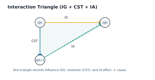
Fig. 18 The interaction triangle. One IG edge (influence), one CST edge (evolution), and one IA edge (attribution) close a single causal loop.#
Let \(m_t := |\mathcal{P}_t|\) be the number of sampled companion pairs at time \(t\).
The following table summarizes the structural properties:
Property |
CST Edges |
IG Edges |
IA Edges |
|---|---|---|---|
Direction |
Timelike (\(t \to t+1\)) |
Spacelike (same \(t\)) |
Diagonal (\(t+1 \to t\)) |
Cardinality |
$\sum_{t=0}^{T-1} |
\mathcal{A}(t) |
$ |
Topology |
Forest (acyclic) |
Directed companion graph per \(t\) |
Bipartite per \((t, t+1)\) on sampled pairs |
Key weight |
Timestep \(\Delta t\) |
Cloning potential \(V_{\mathrm{clone}}\) |
Influence weight \(w_{ij}\) |
Role in triangle |
Evolution edge |
Influence edge |
Attribution edge |
The Big Picture: Why This Structure?
Before diving into the technical details, here is the forest before the trees:
Goal: Recover all declared execution samples from a complete record
Problem: Some quantities (energies) are coordinate-free already; others (velocities, forces) depend on coordinate choice
Solution: Store scalars on nodes and directional payloads on edges and boundary records, with their reference conventions
Bonus: The resulting structure is a directed 2-complex with natural gauge-theoretic properties
The following sections make these ideas precise. Section 1 explains the scalar/vector distinction. Section 2 defines nodes. Section 3 defines temporal edges (CST). Section 4 defines spatial edges (IG). Section 5 puts it all together with influence attribution (IA) edges and triangles. Section 6 specifies complete payload coverage and proves the reconstruction identities. Section 7 shows how it works on curved manifolds. Section 8 gives practical guarantees.
1. Frame Invariance and Covariance#
1.1 Observers and Coordinate Systems#
A coordinate system on the state space \(\mathcal{X} \subseteq \mathbb{R}^d\) is a choice of origin and orthonormal basis \(\{e_1, \ldots, e_d\}\). Two observers using coordinate systems related by a rotation \(R \in \mathrm{SO}(d)\) will represent the same physical configuration differently: if observer 1 assigns coordinates \(x\) to a point, observer 2 assigns coordinates \(x' = Rx\).
Definition 632 (Frame-Invariant Quantity (Scalar))
A quantity \(\phi: \mathcal{X} \to \mathbb{R}\) is frame-invariant (or a scalar field) if its value at any physical point is independent of coordinate choice:
Equivalently, \(\phi' = \phi \circ R^{-1}\) implies \(\phi'(Rx) = \phi(x)\).
Scalars include: kinetic energy \(E_{\mathrm{kin}} = \frac{1}{2}\|v\|^2\), potential energy \(U(x)\), fitness \(\Phi(x)\), distance norms \(\|x - y\|\), and any quantity constructed solely from inner products and norms.
Definition 633 (Frame-Covariant Quantity (Vector))
A quantity \(\mathbf{v}: \mathcal{X} \to \mathbb{R}^d\) is frame-covariant (or a vector field) if its components transform by the same rotation relating the coordinate systems:
Vectors include: position \(x\), velocity \(v\), force \(\mathbf{F}\), gradient \(\nabla\phi\), and any quantity that “points in a direction.”
The key distinction: scalars are the same number in all frames; vectors are the same geometric object but with different numerical components in different frames.
1.2 The Spinor Representation#
Why encode an arrow by a spinor? The useful feature is its transformation law. We can transport the spinor by a spin rotation and then decode the resulting arrow; the answer agrees with rotating the arrow directly.
This does not eliminate bookkeeping. The tuple of complex numbers on disk needs a known spin frame and a known decoder, just as vector components need a known vector frame. The representation makes the relation between frames explicit. It does not let a receiver infer an unspecified frame from the numbers alone.
Vectors transform by \(d \times d\) rotation matrices. For computational and geometric reasons, it is often preferable to represent vectors using spinors—complex objects that transform by a simpler (though higher-dimensional in complex terms) representation.
Definition 634 (Spinor Space)
For state space dimension \(d\), fix a complex spinor module \(\mathbb{S}_d\). For \(d \geq 3\), choose a Clifford representation \(\{\Gamma_i\}_{i=1}^d\) on \(\mathbb{S}_d\). For \(d = 2\), we use the minimal Spin(2) module \(\mathbb{C}\) with the quadratic map \(v = \psi^2\) (already full for \(\mathbb{R}^2\)). For odd \(d\), \(\dim_{\mathbb{C}} \mathbb{S}_d = 2^{(d-1)/2}\). For even \(d \geq 4\), the Dirac module has \(\dim_{\mathbb{C}} = 2^{d/2}\) and splits into two Weyl (chiral) modules; to represent all vectors we use the full Dirac module. A spinor is an element \(\psi \in \mathbb{S}_d\).
The spinor dimension depends on \(d\). We denote \(s_d := \dim_{\mathbb{C}} \mathbb{S}_d\) for the representation chosen for storage. The Fractal Set uses the minimal Spin(2) spinor in \(d = 2\), Dirac spinors in even dimensions \(d \geq 4\) (full vector coverage), and minimal spinors in odd dimensions. Example choices:
Dimension \(d\) |
Storage module \(\mathbb{S}_d\) |
Complex Dimension |
Real Parameters |
Notes |
|---|---|---|---|---|
2 |
\(\mathbb{C}\) |
1 |
2 |
Spin(2) spinor with \(v = \psi^2\) |
3 |
\(\mathbb{C}^2\) |
2 |
4 |
Pauli spinors |
4 |
\(\mathbb{C}^4\) |
4 |
8 |
Dirac spinors (full vector coverage) |
5 |
\(\mathbb{C}^4\) |
4 |
8 |
Minimal odd-dimensional spinor |
6 |
\(\mathbb{C}^8\) |
8 |
16 |
Dirac spinors (full vector coverage) |
7 |
\(\mathbb{C}^8\) |
8 |
16 |
Minimal odd-dimensional spinor |
8 |
\(\mathbb{C}^{16}\) |
16 |
32 |
Dirac spinors (full vector coverage) |
For general \(d\), the Dirac spinor dimension is \(2^{\lfloor d/2 \rfloor}\). Storage and complexity scale with the chosen \(s_d\).
Definition 635 (Spinor Representation of \(\mathrm{SO}(d)\))
The spinor representation is a group homomorphism \(S: \mathrm{Spin}(d) \to \mathrm{GL}(\mathbb{S}_d)\) where \(\mathrm{Spin}(d)\) is the double cover of \(\mathrm{SO}(d)\). For each rotation \(R \in \mathrm{SO}(d)\), there exist exactly two preimages \(\pm U \in \mathrm{Spin}(d)\) such that the equivariant quadratic map \(\pi\) satisfies:
For \(d \geq 3\) (or any Clifford module), \(\pi(\psi)_i = \psi^\dagger \Gamma_i \psi\). For \(d = 2\), \(\pi(\psi) = \psi^2\).
Equivalently, the following diagram commutes:
A vector-to-spinor map \(\iota\) is then a choice of section of \(\pi\) (a gauge-fixing), introduced below.
The sign ambiguity (\(\pm U\) both correspond to \(R\)) reflects the double-cover structure and is a gauge freedom—both choices encode the same physical vector.
Note
The double cover: why \(\pm U\) give the same rotation. Imagine rotating a coffee cup 360 degrees. It returns to its starting position—that is the rotation \(R = I\). But in spinor space, a 360-degree rotation corresponds to \(U = -I\), not \(U = +I\). You need to rotate twice (720 degrees) to get \(U = +I\).
For the geometric encoding here, the double cover means two spinor transformations give the same vector rotation. The later fermionic operator construction specifies its own exterior algebra and stochastic correspondence; the sign under a full rotation alone does not establish those identities.
The gauge freedom is real but harmless: both choices \(\pm U\) produce the same physical answer when you extract vectors from spinors.
1.3 Vector-Spinor Correspondence#
The conversion has two separate jobs: choose an encoding of the vector, and recover the vector from that encoding. In two dimensions the square map has two possible spinor roots. In three dimensions the normalized two-component construction has an entire circle of representatives differing by phase.
In the general Clifford construction, the positive eigenspace of the direction matrix can have dimension greater than one. A deterministic projector-and-pivot rule selects a representative. The freedom is then larger than a phase, and the chosen representative can change discontinuously when the pivot changes. Equivariance belongs to the decoder; it does not assert that this deterministic choice commutes with every rotation.
For storage, the essential identity is the roundtrip: encode an admissible vector using the declared convention, then decode it to recover that vector. These are geometric encoding spinors; their use does not impose a Dirac formulation on the later QFT observables.
The explicit correspondence uses the Clifford algebra \(\mathrm{Cl}(d)\) generated by \(\{e_1, \ldots, e_d\}\) with \(e_i e_j + e_j e_i = 2\delta_{ij}\). We use the Euclidean convention so the representing matrices \(\Gamma_i\) can be taken Hermitian, which makes \(\psi^\dagger \Gamma_i \psi\) real.
Definition 636 (Vector-to-Spinor Map)
The vector-to-spinor embedding \(\iota: \mathbb{R}^d \to \mathbb{S}_d\) encodes vectors as spinors with a specified representative convention. For \(v = \sum_i v_i e_i \in \mathbb{R}^d\):
Case \(d = 2\): Spinor square representation. Write \(v = v_1 + i v_2 = r e^{i\phi}\) with \(\phi \in (-\pi, \pi]\) and define
Then the extraction map is \(\pi(\psi) = \psi^2\), so \(\pi(\iota(v)) = v\). The phase convention fixes the sign ambiguity of the square root.
Case \(d = 3\): Using the canonical lift with real first component when possible,
where \((\|v\|, \theta, \phi)\) are spherical coordinates: \(v = \|v\|(\sin\theta\cos\phi, \sin\theta\sin\phi, \cos\theta)\).
Equivalently, for \(v \neq 0\): construct the Hermitian matrix \(v \cdot \boldsymbol{\sigma} = v_1 \sigma_1 + v_2 \sigma_2 + v_3 \sigma_3\) and take the eigenvector with eigenvalue \(+\|v\|\), normalized to have \(\|\psi\|^2 = \|v\|\) and first component real non-negative.
For \(v = 0\): \(\iota(0) = 0\) in any dimension.
General \(d\geq3\): For \(v\ne0\), set \(r=\|v\|\), \(n=v/r\), and \(P_+(n)=(I+n\cdot\Gamma)/2\). In the fixed orthonormal basis \((e_a)\) of \(\mathbb S_d\), let \(a(n)\) be the first index maximizing \(\|P_+(n)e_a\|\) and set
This prescription fixes the representative in the entire positive eigenspace. For \(d=3\) one may instead use the displayed spherical section, taking \(\iota(0,0,-r)=\sqrt r(0,1)^{\mathsf T}\) at its exceptional pole. The selected section is part of the serialization convention.
Remark: The projector section is measurable and smooth wherever its selected pivot remains fixed. Since \(\operatorname{tr}P_+=s_d/2\), its maximal column has squared norm at least \(1/2\). Thus its normalization is defined for every nonzero \(v\). The Pauli section in \(d=3\) has the familiar Hopf-fibration patch transition. Higher-dimensional positive eigenspaces can have dimension greater than one; a phase alone does not select their representatives.
Definition 637 (Spinor-to-Vector Map)
The spinor-to-vector extraction \(\pi: \mathbb{S}_d \to \mathbb{R}^d\) is the left inverse of \(\iota\) (on the image of \(\iota\)):
Case \(d = 2\): For \(\psi \in \mathbb{C}\) identified with \(\mathbb{R}^2\),
Case \(d = 3\): For \(\psi = \begin{pmatrix} \alpha \\ \beta \end{pmatrix} \in \mathbb{C}^2\),
General \(d \geq 3\): With a fixed Clifford representation \(\{\Gamma_i\}\),
which is equivariant under \(\mathrm{Spin}(d)\) and reduces to the low-dimensional formulas above.
Lemma 272 (Exact vector encoding and its frame convention)
The section in Definition 636 satisfies \(\pi\circ\iota=\mathrm{id}_{\mathbb R^d}\). Its numerical representation includes the chosen Clifford matrices, spinor basis, physical frame, units, and section rule. In a manifold chart it also includes the chart and local frame identifiers.
Proof. The \(d=2\) assertion is \((\sqrt r e^{i\phi/2})^2=re^{i\phi}\). For \(d\geq3\), the Clifford relations give \((n\cdot\Gamma)^2=I\) and \(P_+^2=P_+=P_+^\dagger\). Put \(u=P_+e_a/\|P_+e_a\|\). Then \((n\cdot\Gamma)u=u\) and \(\|u\|=1\). Write \(e_j=n_jn+w_j\) with \(w_j\perp n\). Anticommutation gives
Consequently \(\iota(v)^\dagger\Gamma_j\iota(v)=rn_j=v_j\). At zero both sides vanish. The coordinate components are interpreted in the recorded frame; rotation to another frame uses its known transition map. \(\square\)
Definition 638 (Matrix encoding by spinor columns)
For a real \(d\times d\) matrix \(A\) in specified output and input frames, define
Then \(\mathcal P_2\mathcal I_2(A)=A\) column by column by Lemma 272. The code stores \(d s_d\) complex components, with their frame convention. For diffusion amplitudes the input frame is the noise frame. A change of output and input frames gives \(A'=R_{\mathrm{out}}AR_{\mathrm{in}}^{\mathsf T}\); encoding \(A'\) uses these transformed columns. This specifies the tensor decoder used below.
Proposition 205 (Transformation Covariance)
For \(R\in\mathrm{SO}(d)\) and its spinor lift \(U\), represented on \(\mathbb S_d\),
Both \(U\iota(v)\) and \(\iota(Rv)\) decode to \(Rv\). In \(d=2\) they differ by a sign, and in \(d=3\) nonzero representatives differ by a unit phase. In general they lie in the same decoder fiber, which can be larger than a phase orbit.
Proof. For \(d\geq3\), use \(U^\dagger\Gamma_jU=\sum_kR_{jk}\Gamma_k\) in the quadratic decoder. For \(d=2\), \(U=e^{i\theta/2}\) gives \((U\psi)^2=e^{i\theta}\psi^2\). The second identity follows from Lemma 272. The positive eigenspace of \(n\cdot\Gamma\) has dimension \(s_d/2\); when this is greater than one, its unit vectors need not be phase multiples. \(\square\)
Think of the decoder as a calibrated instrument. Its frame and Clifford convention tell you what its readings mean. Change the frame consistently and the readings describe the rotated arrow, with the same norm and scalar contractions. Discard the calibration and the stored components are no longer enough to identify that arrow.
This is why the serialization includes reference conventions. Coordinate covariance is a relation between complete descriptions in different frames.
2. Nodes: Spacetime Points with Scalar Data#
A node identifies a walker at a recorded stage and stores scalar measurements such as fitness and status. Directional data are carried by the edge payloads and associated boundary records.
This is a storage convention that makes transformation rules easy to check. It does not mean that scalars alone determine a walker’s instantaneous state: position and velocity still have to be recovered from their recorded covariant data.
2.1 Node Set Definition#
Definition 639 (Spacetime Node)
A spacetime node \(n_{i,t}\) represents walker \(i \in \{1, \ldots, N\}\) at discrete timestep \(t \in \{0, 1, \ldots, T\}\). The node set is:
The cardinality is \(|\mathcal{N}| = N(T+1)\).
Each node represents a single “event” in the algorithm’s spacetime: a specific walker at a specific moment. The node set forms a rectangular grid \(\{1, \ldots, N\} \times \{0, \ldots, T\}\), though connectivity (via edges) respects the actual alive/dead status of walkers.
2.2 Node Scalar Attributes#
Nodes store only scalar quantities—values that are frame-invariant.
Definition 640 (Node Scalar Attributes)
Each node \(n_{i,t} \in \mathcal{N}\) carries the following scalar attributes:
Identity attributes:
Attribute |
Symbol |
Type |
Unit |
Description |
|---|---|---|---|---|
Walker ID |
\(\mathrm{id}(n)\) |
\(\mathbb{Z}_+\) |
[count] |
Unique identifier for walker |
Timestep |
\(t(n)\) |
\(\mathbb{Z}_{\geq 0}\) |
[count] |
Discrete time index |
Node ID |
\(\mathrm{nid}(n)\) |
\(\mathbb{Z}_+\) |
[count] |
Unique identifier for node |
Temporal attributes:
Attribute |
Symbol |
Type |
Unit |
Description |
|---|---|---|---|---|
Algorithmic time |
\(\tau(n)\) |
\(\mathbb{R}_{\geq 0}\) |
[time] |
Continuous time: \(\tau = t \cdot \Delta t\) |
Timestep duration |
\(\Delta t\) |
\(\mathbb{R}_{>0}\) |
[time] |
Time between consecutive steps |
Status attributes:
Attribute |
Symbol |
Type |
Unit |
Description |
|---|---|---|---|---|
Alive flag |
\(s(n)\) |
\(\{0, 1\}\) |
[boolean] |
1 if walker alive at this timestep, 0 otherwise |
Clone source |
\(c(n)\) |
\(\mathbb{Z}_+ \cup \{\bot\}\) |
[count] |
ID of cloning source if cloned this step, \(\bot\) otherwise |
Energy attributes:
Attribute |
Symbol |
Type |
Unit |
Description |
|---|---|---|---|---|
Kinetic energy |
\(E_{\mathrm{kin}}(n)\) |
\(\mathbb{R}_{\geq 0}\) |
[energy] |
\(\frac{1}{2}|v|^2\) at this node |
Potential energy |
\(U(n)\) |
\(\mathbb{R}\) |
[energy] |
Potential energy \(U(x)\) at position |
Total energy |
\(E(n)\) |
\(\mathbb{R}\) |
[energy] |
\(E_{\mathrm{kin}}(n) + U(n)\) |
Fitness attributes:
Attribute |
Symbol |
Type |
Unit |
Description |
|---|---|---|---|---|
Fitness |
\(\Phi(n)\) |
\(\mathbb{R}_{\geq 0}\) |
[dimensionless] |
Objective function value \(\Phi(x)\) |
Virtual reward |
\(V_{\mathrm{fit}}(n)\) |
\(\mathbb{R}\) |
[dimensionless] |
Localized fitness potential \(V_{\mathrm{fit}}[f_k, \rho](x)\) |
Reward signal |
\(r(n)\) |
\(\mathbb{R}\) |
[dimensionless] |
Instantaneous reward (if applicable) |
Localized statistics:
Attribute |
Symbol |
Type |
Unit |
Description |
|---|---|---|---|---|
Local mean |
\(\mu_\rho(n)\) |
\(\mathbb{R}\) |
[dimensionless] |
Kernel-weighted mean fitness around \(x\) |
Local std |
\(\sigma_\rho(n)\) |
\(\mathbb{R}_{\geq 0}\) |
[dimensionless] |
Kernel-weighted std of fitness |
Local derivative |
\(\sigma'_\rho(n)\) |
\(\mathbb{R}\) |
[1/distance] |
Derivative of \(\sigma_\rho\) w.r.t. \(\rho\) |
Partition function |
\(Z_\rho(n)\) |
\(\mathbb{R}_{>0}\) |
[dimensionless] |
Normalizing constant for kernel |
Global parameters (constant across nodes):
Attribute |
Symbol |
Type |
Unit |
Description |
|---|---|---|---|---|
Fermi energy |
\(\epsilon_F\) |
\(\mathbb{R}\) |
[energy] |
Selection threshold parameter |
Viscosity |
\(\nu\) |
\(\mathbb{R}_{\geq 0}\) |
[1/time] |
Viscous coupling strength |
Friction |
\(\gamma\) |
\(\mathbb{R}_{\geq 0}\) |
[1/time] |
Velocity damping coefficient |
Localization scale |
\(\rho\) |
\(\mathbb{R}_{>0}\) |
[distance] |
Kernel bandwidth |
Diffusion floor |
\(\epsilon_\Sigma\) |
\(\mathbb{R}_{>0}\) |
[dimensionless] |
Regularization for diffusion tensor |
Definition 641 (Clone Ancestry Relation)
The clone ancestry graph is the derived directed relation
This encodes genealogical branching (parent \(j\) to child \(i\)) and can be read directly from the clone source attribute or from IA edges with \(\chi_{\mathrm{clone}}=1\). These edges are not part of the CST order or distance; they are interaction/genealogy data only.
2.3 Frame-Invariance of Node Data#
Proposition 206 (Node Scalars are Frame-Invariant)
Every attribute in Definition 640 is a scalar field in the sense of Definition 632.
Proof. Each attribute falls into one of the following categories:
Discrete identifiers (\(\mathrm{id}\), \(t\), \(\mathrm{nid}\), \(s\), \(c\)): Pure labels with no geometric content.
Time coordinates (\(\tau\), \(\Delta t\)): Time is a scalar (same in all spatial coordinate systems under \(\mathrm{SO}(d)\)).
Norms and scalar fields (\(E_{\mathrm{kin}} = \frac{1}{2}\|v\|^2\), \(U(x)\), \(\Phi(x)\), \(V_{\mathrm{fit}}\)): Norms are invariant, and scalar fields assign coordinate-independent values to points.
Statistical aggregates (\(\mu_\rho\), \(\sigma_\rho\), \(Z_\rho\)): Defined via integration over scalar kernels.
Constants (\(\epsilon_F\), \(\nu\), \(\gamma\), \(\rho\), \(\epsilon_\Sigma\)): Parameters independent of position or orientation.
None of these scalar quantities depend on coordinate choice. \(\square\)
The scalar node attributes summarize the recorded state, while the directional payloads determine its position, velocity, and evaluated forces in the declared frame. Both parts are needed for reconstruction. In particular, a node with no suitable incident payload needs a boundary record; its fitness and energy cannot supply a missing position.
A slot is not an ancestor

Rust engine experiment · Seed 7 · Poster after 11 experiment steps. Interactive view starts from the same seed.
3. CST Edges: Temporal Evolution with Spinor Data#
3.1 Edge Set Definition#
Definition 642 (CST Edge Set)
The Causal Spacetime Tree (CST) edge set is:
Each CST edge connects a walker to its immediate temporal successor, provided the walker is alive. The edges are directed from earlier to later time.
Under this coarse node convention, CST edges form directed paths of walker slots, interrupted where the source alive flag is zero. A cloning event changes the state occupying a slot; the displayed edge rule does not cut the path at that event. Clone-source pointers separately record genealogy. The stage-resolved record in Definition 661 distinguishes the pre-cloning, post-cloning, and post-kinetic states and the corresponding updates.
Definition 643 (Alive Walker Set)
At timestep \(t\), the alive walker set is:
The number of alive walkers is \(k_t := |\mathcal{A}(t)|\).
The number of allocated walker slots is \(N\), while \(0\leq k_t\leq N\) is computed from the recorded alive mask. A revival update can change that mask; slot persistence alone does not set \(k_t=N\). For the killed convention, \(k_t<2\) ends the nonabsorbing evolution as specified in Definition 497 and the algorithm’s companion rule.
3.2 Causal Set Axioms#
Following CST edges always advances the algorithmic clock. Their reachability relation therefore gives a finite causal order. This is a useful exact statement about the execution graph.
Recovering continuum geometry requires more information than these finite-order axioms. Volume 2 already develops that information: fitness regularity controls the constructed metric, the graph-distance comparison transfers edge accuracy and path coverage to distance accuracy, and joint-law LSI/Poincaré estimates control sampling fluctuations. See Lemma 295 and Lemma 298.
The order and clock must still be identified with the geometric objects used by those theorems. Algorithmic time counts updates. Proper time, when the Lorentzian construction applies, is computed along the reconstructed trajectory with its metric; it is not automatically the same clock.
The transitive closure of the CST edges is a locally finite strict partial order.
Definition 644 (Causal Set Axioms)
A causal set is a pair \((\mathcal{C}, \prec)\) where \(\mathcal{C}\) is a set and \(\prec\) is a binary relation satisfying:
CS1 (Irreflexivity): \(\forall x \in \mathcal{C}: \neg(x \prec x)\). No element is its own ancestor.
CS2 (Transitivity): \(\forall x, y, z \in \mathcal{C}: (x \prec y \land y \prec z) \Rightarrow x \prec z\). The ancestor relation is transitive.
CS3 (Local Finiteness): \(\forall x, z \in \mathcal{C}: |\{y \in \mathcal{C} : x \prec y \prec z\}| < \infty\). Causal intervals contain finitely many elements.
Proposition 207 (CST Satisfies Causal Set Axioms)
Define the causal relation \(\prec_{\mathrm{CST}}\) on \(\mathcal{N}\) as the transitive closure of \(E_{\mathrm{CST}}\):
Then \((\mathcal{N}, \prec_{\mathrm{CST}})\) satisfies CS1, CS2, and CS3.
Proof.
CS1 (Irreflexivity): CST edges always increase the timestep: \((n_{i,t}, n_{i,t+1})\) has \(t+1 > t\). Any path in \(E_{\mathrm{CST}}\) strictly increases the timestep, so no path can return to its starting node. Thus \(\neg(n \prec_{\mathrm{CST}} n)\) for all \(n\).
CS2 (Transitivity): By definition, \(\prec_{\mathrm{CST}}\) is the transitive closure, hence transitive.
CS3 (Local Finiteness): If \(n_{i,t} \prec_{\mathrm{CST}} n_{j,s}\), then \(t < s\). The causal interval \(\{n : n_{i,t} \prec_{\mathrm{CST}} n \prec_{\mathrm{CST}} n_{j,s}\}\) contains only nodes with timesteps in \(\{t+1, \ldots, s-1\}\), which is finite. Moreover, at each timestep there are at most \(N\) walkers. Thus the interval has at most \(N(s-t-1) < \infty\) elements. \(\square\)
The CST order describes which recorded updates precede others. IA arrows point backward to identify sources, but they are not added to the forward CST order. Keeping these roles separate prevents an attribution loop from being mistaken for a causal-order cycle.
3.3 CST Edge Spinor Attributes#
Each CST edge stores the spinor representations of all vectorial quantities involved in the temporal evolution.
Definition 645 (CST Edge Spinor Attributes)
Each CST edge \(e = (n_{i,t}, n_{i,t+1}) \in E_{\mathrm{CST}}\) carries the following attributes:
Identity attributes:
Attribute |
Symbol |
Type |
Unit |
Description |
|---|---|---|---|---|
Walker ID |
\(\mathrm{id}(e)\) |
\(\mathbb{Z}_+\) |
[count] |
Walker this edge belongs to |
Start timestep |
\(t(e)\) |
\(\mathbb{Z}_{\geq 0}\) |
[count] |
Timestep of source node |
Edge ID |
\(\mathrm{eid}(e)\) |
\(\mathbb{Z}_+\) |
[count] |
Unique edge identifier |
Velocity spinors:
Attribute |
Symbol |
Type |
Unit |
Description |
|---|---|---|---|---|
Initial velocity |
\(\psi_{v,t}(e)\) |
\(\mathbb{S}_d\) |
[distance/time] |
Spinor of \(v_i(t)\) |
Final velocity |
\(\psi_{v,t+1}(e)\) |
\(\mathbb{S}_d\) |
[distance/time] |
Spinor of \(v_i(t+1)\) |
Velocity increment |
\(\psi_{\Delta v}(e)\) |
\(\mathbb{S}_d\) |
[distance/time] |
Spinor of \(\Delta v = v_i(t+1) - v_i(t)\) |
Position spinor:
Attribute |
Symbol |
Type |
Unit |
Description |
|---|---|---|---|---|
Displacement |
\(\psi_{\Delta x}(e)\) |
\(\mathbb{S}_d\) |
[distance] |
Spinor of \(\Delta x = x_i(t+1) - x_i(t)\) |
Force spinors:
Attribute |
Symbol |
Type |
Unit |
Description |
|---|---|---|---|---|
Stable force |
\(\psi_{\mathbf{F}_{\mathrm{stable}}}(e)\) |
\(\mathbb{S}_d\) |
[distance/time^2] |
Spinor of \(\mathbf{F}_{\mathrm{stable}}(x_i)\) |
Adaptive force |
\(\psi_{\mathbf{F}_{\mathrm{adapt}}}(e)\) |
\(\mathbb{S}_d\) |
[distance/time^2] |
Spinor of \(\mathbf{F}_{\mathrm{adapt}}(x_i, S)\) |
Viscous force |
\(\psi_{\mathbf{F}_{\mathrm{viscous}}}(e)\) |
\(\mathbb{S}_d\) |
[distance/time^2] |
Spinor of \(\mathbf{F}_{\mathrm{viscous}}(x_i, S)\) |
Friction force |
\(\psi_{\mathbf{F}_{\mathrm{friction}}}(e)\) |
\(\mathbb{S}_d\) |
[distance/time^2] |
Spinor of \(-\gamma v_i\) |
Total force |
\(\psi_{\mathbf{F}_{\mathrm{total}}}(e)\) |
\(\mathbb{S}_d\) |
[distance/time^2] |
Spinor of \(\mathbf{F}_{\mathrm{total}} = \sum \mathbf{F}_{\cdot}\) |
Diffusion spinors:
Attribute |
Symbol |
Type |
Unit |
Description |
|---|---|---|---|---|
Diffusion tensor |
\(\psi_{\Sigma_{\mathrm{reg}}}(e)\) |
\((\mathbb{S}_d)^d\) |
[distance/time^{3/2}] |
Column encoding \(\mathcal I_2(\Sigma_{\mathrm{reg}})\) |
Noise realization |
\(\psi_{\mathrm{noise}}(e)\) |
\(\mathbb{S}_d\) |
[distance/time] |
Spinor of the stochastic increment \(\Sigma_{\mathrm{reg}} \circ dW_i\) |
Gradient spinors:
Attribute |
Symbol |
Type |
Unit |
Description |
|---|---|---|---|---|
Potential gradient |
\(\psi_{\nabla U}(e)\) |
\(\mathbb{S}_d\) |
[energy/distance] |
Spinor of \(\nabla U(x_i)\) |
Fitness gradient |
\(\psi_{\nabla \Phi}(e)\) |
\(\mathbb{S}_d\) |
[1/distance] |
Spinor of \(\nabla \Phi(x_i)\) |
Virtual reward gradient |
\(\psi_{\nabla V_{\mathrm{fit}}}(e)\) |
\(\mathbb{S}_d\) |
[1/distance] |
Spinor of \(\nabla V_{\mathrm{fit}}(x_i)\) |
Derived scalars (stored for efficiency):
Attribute |
Symbol |
Type |
Unit |
Description |
|---|---|---|---|---|
Velocity norm change |
\(|\Delta v|(e)\) |
\(\mathbb{R}_{\geq 0}\) |
[distance/time] |
\(|\Delta v|\) |
Displacement norm |
\(|\Delta x|(e)\) |
\(\mathbb{R}_{\geq 0}\) |
[distance] |
\(|\Delta x|\) |
Timestep |
\(\Delta t(e)\) |
\(\mathbb{R}_{>0}\) |
[time] |
Time duration of this step |
Remark 242 (Payload units and evaluation stages)
The unit column in the vector and matrix tables gives the unit of the decoded quantity. Since \(\pi\) is quadratic, \([\iota(v)]=[v]^{1/2}\), and each column of \(\mathcal I_2(A)\) has unit \([A]^{1/2}\). Every force and noise payload carries its evaluation-stage identifier. Endpoint state data and intermediate force evaluations are distinct samples of the split update.
3.4 Relationship to SDE Dynamics#
The CST edge data encodes one complete step of the stochastic differential equation governing walker dynamics. The variant used here is the Geometric Gas (Definition 424), whose defining dynamics are the geometric kinetic dynamics Definition 621 of The Geometric Gas: Regularity, Stability, and Entropy.
Definition 646 (Geometric Gas SDE)
In the notation of this chapter, the dynamics of the Geometric Gas (Definition 424) for walker \(i\) with state \((x_i, v_i)\) take the form:
where:
\(\mathbf{F}_{\mathrm{stable}}(x) = -\nabla U(x)\) is the conservative force from the potential
\(\mathbf{F}_{\mathrm{adapt}}(x, S) = -\nabla V_{\mathrm{fit}}[f_k, \rho](x)\) is the adaptive force from the fitness landscape
\(\mathbf{F}_{\mathrm{viscous}}(x, S) = \nu \sum_{j \neq i} K_\rho(x_i, x_j)(v_j - v_i)\) is the viscous coupling force
\(\Sigma_{\mathrm{reg}}(x, S)\) is the fitness-adapted diffusion tensor
\(dW_i\) is a standard Wiener process
The variant itself is defined by Definition 621, which uses row-normalized viscous weights and the adaptive force \(\epsilon_F\nabla_{x_i}V_i\); the two conventions are compared in Definition 424.
Compare this equation with Definition 621 term by term and you will find the same four forces plus the same fitness-adapted Stratonovich noise. Only the bookkeeping differs: here the viscous coupling is written with the raw kernel weights \(K_\rho(x_i,x_j)\) and the adaptive force as \(-\nabla V_{\mathrm{fit}}\), while Definition 621 uses the row-normalized weights \(W_{ij}=K_{ij}/\sum_{l\ne i}K_{il}\) and \(F_i=\epsilon_F\nabla_{x_i}V_i\). The comparison is made explicit in Definition 424.
That distinction matters for what you may claim. The convergence results of The Geometric Gas: Regularity, Stability, and Entropy are proved for the normalized convention, and each one carries its own hypotheses — the spectral margin, the cloning estimate, the viscous degree comparison. Writing the same physics with unnormalized weights does not by itself transport those theorems here; you must identify the constants first. For this chapter nothing is lost, because all we need of the SDE is its shape: which quantities a CST edge has to store so that one step can be replayed exactly.
Notice also the word “adaptive” in \(\mathbf{F}_{\mathrm{adapt}}\) and in the adaptive diffusion tensor \(\Sigma_{\mathrm{reg}}\). That is a description of what those objects do — they follow the measured fitness landscape — not the name of a gas variant. The variant is the Geometric Gas.
Proposition 208 (CST Edge Encodes Complete Kinetic Update)
Given the CST edge attributes for \(e = (n_{i,t}, n_{i,t+1})\), the complete evolution from \((x_i(t), v_i(t))\) to \((x_i(t+1), v_i(t+1))\) can be reconstructed:
and all force components:
Proof. By Proposition 205, the spinor-to-vector map \(\pi\) recovers the geometric vector from its spinor representation. The spinor attributes store exactly the quantities appearing in the SDE Definition 646. \(\square\)
Read a CST payload as a record of a specified transition. Together with its starting-state anchor, stage conventions, and recorded updates, it determines the corresponding endpoint. Forces are recovered at the evaluation stages actually stored; a terminal evaluation belongs in a boundary record when there is no outgoing edge.
Two observers using consistently transformed reference frames recover correspondingly transformed trajectories. The exact statement is algebraic in real arithmetic. Floating-point decoding introduces errors determined by precision and conditioning.
3.5 Spinor Operations Complexity#
Proposition 209 (Spinor Conversion Complexity)
The vector-to-spinor map \(\iota: \mathbb{R}^d \to \mathbb{S}_d\) and spinor-to-vector map \(\pi: \mathbb{S}_d \to \mathbb{R}^d\) have dimension-dependent complexity:
Dimension \(d\) |
\(\iota\) Time |
\(\pi\) Time |
Spinor Storage |
|---|---|---|---|
2 |
\(O(1)\) |
\(O(1)\) |
2 reals |
3 |
\(O(1)\) |
\(O(1)\) |
4 reals |
4 |
\(O(1)\) |
\(O(1)\) |
8 reals |
General |
\(O(s^3)\) |
\(O(d\,s^2)\) |
\(2s\) reals where \(s = \dim_{\mathbb{C}}\mathbb{S}_d\) |
For \(d \leq 4\), conversions are constant-time with fixed arithmetic operations. For general \(d\), the eigenvector computation in \(\iota\) is \(O(s^3)\) in the worst case for an \(s \times s\) Hermitian matrix, while \(\pi\) (the bilinear forms \(\psi^\dagger \Gamma_i \psi\)) is \(O(s^2)\) per component, giving \(O(d\,s^2)\) total. Sparse Clifford representations can reduce constants.
Proof. For \(d = 2\): constant-time complex square root/extraction. For \(d = 3\): trigonometric functions and 2×2 matrix operations. For general \(d\): eigenvalue decomposition of \(s \times s\) Hermitian matrix. \(\square\)
4. IG Edges: Asymmetric Selection Coupling#
4.1 Edge Set Definition#
Definition 647 (IG Edge Set)
Let \(\mathcal{P}_t\) be the set of ordered companion pairs realized at timestep \(t\) by the companion selection operators (distance and cloning; Definition 663). The Information Graph (IG) edge set is:
Each IG edge connects an ordered sampled pair of distinct alive walkers at the same timestep. The edges are directed: by convention, \((n_{i,t}, n_{j,t})\) is oriented from the influenced walker \(i\) toward the influencer \(j\). Edges at \(t = T\) are terminal-time snapshots and do not participate in IA edges or triangles.
Proposition 210 (IG Edge Cardinality)
At timestep \(t\) with \(k_t = |\mathcal{A}(t)|\) alive walkers, the number of IG edges is \(m_t := |\mathcal{P}_t|\). The total across all timesteps is:
Proof. Each sampled ordered pair \((i, j) \in \mathcal{P}_t\) contributes one edge. \(\square\)
For the sequential greedy pairing operator (Definition 529), \(m_t = k_t - f_t\) with \(f_t \in \{0,1\}\) fixed points. In general, the IG edges at each timestep form a directed companion graph on the alive walkers, restricted to the sampled pairs; the influence is asymmetric, so the edge \((i, j)\) need not imply \((j, i)\) unless the pairing is mutual.
4.2 Directionality and Antisymmetry#
The key structural property of IG edges is the antisymmetry of the cloning potential.
Definition 648 (Directed Cloning Potential)
The directed cloning potential from walker \(i\) to walker \(j\) at timestep \(t\) is:
where \(\Phi_i(t) := \Phi(n_{i,t})\) is the fitness of walker \(i\) at time \(t\).
Proposition 211 (Antisymmetry of Cloning Potential)
The cloning potential is antisymmetric under exchange of walkers:
Proof. Direct computation:
This antisymmetry has profound implications:
Corollary 111 (Selection Asymmetry)
If \(\Phi_j(t) > \Phi_i(t)\) (walker \(j\) is fitter than walker \(i\)), then:
\(V_{\mathrm{clone}}(i \to j; t) > 0\): Walker \(i\) is “pulled toward” walker \(j\) (wants to clone from \(j\))
\(V_{\mathrm{clone}}(j \to i; t) < 0\): Walker \(j\) is “pushed away” from walker \(i\) (does not want to clone from \(i\))
The cloning potential biases flow from less fit to more fit; realized cloning events can still be stochastic or constrained by other rules.
A directed score tells us which way selection favors copying. To see how these data enter a fermionic construction, keep track of the operator assigned to an edge. In Theorem 342, the matrix unit for an edge becomes the bilinear \(a_i^\dagger a_j\): it removes occupation from mode \(j\) and adds occupation to mode \(i\). Summing with the recorded coefficients gives \(d\Gamma(A)=\sum_{ij}A_{ij}a_i^\dagger a_j\). This operator preserves the total occupation number. The edge supplies its coefficient; the creation and annihilation operators act on the exterior space.
The antisymmetric part of a real edge matrix, \(A=K-K^\top\), has a precise consequence: \(iA\) is Hermitian. Its second quantization therefore generates a finite-dimensional unitary evolution. This gives an explicit operator construction from the directed record, with every matrix element specified.
There is also an exact connection to stochastic evolution. Theorem 340 identifies the fermionic Fock sectors over the centered space \(L^2_0(\pi)\) with the corresponding centered antisymmetric sector of independent replicas of the process. Evolving each replica carries these functions into one another exactly as the exterior-power evolution prescribes. Independence matters here: a replica is another copy of the process, so this identity does not identify arbitrary correlations between interacting walkers in one swarm with fermionic correlations. The theorem specifies the states and dynamics for which the identification holds.
4.3 IG Edge Spinor Attributes#
Definition 649 (IG Edge Spinor Attributes)
Each IG edge \(e = (n_{i,t}, n_{j,t}) \in E_{\mathrm{IG}}\) carries the following attributes:
Identity attributes:
Attribute |
Symbol |
Type |
Unit |
Description |
|---|---|---|---|---|
Source walker |
\(i(e)\) |
\(\mathbb{Z}_+\) |
[count] |
Walker being influenced |
Target walker |
\(j(e)\) |
\(\mathbb{Z}_+\) |
[count] |
Walker exerting influence |
Timestep |
\(t(e)\) |
\(\mathbb{Z}_{\geq 0}\) |
[count] |
Timestep of interaction |
Edge ID |
\(\mathrm{eid}(e)\) |
\(\mathbb{Z}_+\) |
[count] |
Unique edge identifier |
Position spinors:
Attribute |
Symbol |
Type |
Unit |
Description |
|---|---|---|---|---|
Source position |
\(\psi_{x_i}(e)\) |
\(\mathbb{S}_d\) |
[distance] |
Spinor of \(x_i(t)\) |
Target position |
\(\psi_{x_j}(e)\) |
\(\mathbb{S}_d\) |
[distance] |
Spinor of \(x_j(t)\) |
Relative position |
\(\psi_{\Delta x_{ij}}(e)\) |
\(\mathbb{S}_d\) |
[distance] |
Spinor of \(x_j - x_i\) |
Velocity spinors:
Attribute |
Symbol |
Type |
Unit |
Description |
|---|---|---|---|---|
Source velocity |
\(\psi_{v_i}(e)\) |
\(\mathbb{S}_d\) |
[distance/time] |
Spinor of \(v_i(t)\) |
Target velocity |
\(\psi_{v_j}(e)\) |
\(\mathbb{S}_d\) |
[distance/time] |
Spinor of \(v_j(t)\) |
Relative velocity |
\(\psi_{\Delta v_{ij}}(e)\) |
\(\mathbb{S}_d\) |
[distance/time] |
Spinor of \(v_j - v_i\) |
Coupling spinors:
Attribute |
Symbol |
Type |
Unit |
Description |
|---|---|---|---|---|
Viscous coupling |
\(\psi_{\mathrm{viscous}, ij}(e)\) |
\(\mathbb{S}_d\) |
[distance/time^2] |
Spinor of \(\nu K_\rho(x_i, x_j)(v_j - v_i)\) |
Scalar attributes:
Attribute |
Symbol |
Type |
Unit |
Description |
|---|---|---|---|---|
Kernel weight |
\(K_\rho(e)\) |
\(\mathbb{R}_{\geq 0}\) |
[dimensionless] |
\(K_\rho(x_i, x_j) = \exp(-|x_i - x_j|^2 / 2\rho^2)\) |
Normalized weight |
\(w_{ij}(e)\) |
\(\mathbb{R}_{\geq 0}\) |
[probability] |
\(w_{ij} = K_\rho(e) / \sum_{l \in \mathcal{A}(t) \setminus \{i\}} K_\rho(x_i, x_l)\) |
Euclidean distance |
\(d_{ij}(e)\) |
\(\mathbb{R}_{\geq 0}\) |
[distance] |
\(|x_i - x_j|\) |
Algorithmic distance |
\(d_{\mathrm{alg}, ij}(e)\) |
\(\mathbb{R}_{\geq 0}\) |
[distance] |
\(\sqrt{|x_i - x_j|^2 + \lambda_{\mathrm{alg}}|v_i - v_j|^2}\) |
Phase potential |
\(\theta_{ij}(e)\) |
\(\mathbb{R}\) |
[dimensionless] |
\(-(\Phi_j - \Phi_i)/\hbar_{\mathrm{eff}}\) |
Source fitness |
\(\Phi_i(e)\) |
\(\mathbb{R}_{\geq 0}\) |
[dimensionless] |
\(\Phi(x_i)\) |
Target fitness |
\(\Phi_j(e)\) |
\(\mathbb{R}_{\geq 0}\) |
[dimensionless] |
\(\Phi(x_j)\) |
Cloning potential |
\(V_{\mathrm{clone}}(e)\) |
\(\mathbb{R}\) |
[dimensionless] |
\(\Phi_j - \Phi_i\) (antisymmetric) |
Complex amplitude (optional):
Attribute |
Symbol |
Type |
Unit |
Description |
|---|---|---|---|---|
Coupling amplitude |
\(\psi_{ij}(e)\) |
\(\mathbb{C}\) |
[probability^{1/2}] |
\(\sqrt{P_{\mathrm{comp}}(i,j)} \cdot e^{i\theta_{ij}}\) |
4.4 Viscous Coupling Representation#
Now let us talk about viscosity. In a real gas, molecules that are close together tend to drag each other along—fast molecules slow down, slow molecules speed up, and the gas develops a kind of internal friction. This is viscosity: the tendency of nearby particles to share momentum.
The Fractal Gas has the same effect, but it is engineered rather than emergent. When walker \(i\) is near walker \(j\), they exchange momentum through a viscous coupling force. The force is proportional to the velocity difference \((v_j - v_i)\)—if \(j\) is moving faster, it pulls \(i\) along; if \(j\) is slower, it drags \(i\) back.
The strength of this coupling falls off with distance through the kernel \(K_\rho(x_i, x_j) = \exp(-\|x_i - x_j\|^2 / 2\rho^2)\). Nearby walkers couple strongly; distant walkers barely feel each other. This is how the algorithm creates local coherence without global rigidity.
Why do we want this? Because optimization benefits from coherent exploration. If all walkers in a region are moving in roughly the same direction, they can explore that direction efficiently. Without viscosity, walkers would scatter chaotically and waste computational effort. With viscosity, they form something like a flock of birds—individually free, but collectively coordinated.
The viscous force creates momentum exchange between nearby walkers.
Definition 650 (Pairwise Viscous Force)
The pairwise viscous force exerted by walker \(j\) on walker \(i\) is:
where \(K_\rho(x, y) := \exp(-\|x - y\|^2 / 2\rho^2)\) is the Gaussian kernel with bandwidth \(\rho\).
The total viscous force on walker \(i\) is:
Proposition 212 (Viscous Force Reconstruction from IG Edges)
Define the IG-restricted viscous interaction for walker \(i\) at timestep \(t\):
If the viscous coupling is evaluated on the sampled companion graph, then \(\mathbf{F}_{\mathrm{viscous}}^{\mathrm{IG}} = \mathbf{F}_{\mathrm{viscous}}\). In the full-kernel variant of Definition 650, the total force is recomputed directly from node data using the kernel definition, and the applied total is stored on the CST edge.
Proof. Each IG edge \((n_{i,t}, n_{j,t})\) stores the spinor \(\psi_{\mathrm{viscous}, ij}\) of the pairwise force for that sampled pair. Summing over IG edges with source \(i\) yields the interaction recorded on the sampled graph. \(\square\)
4.5 Algorithmic Distance and Fitness Phase#
The Latent Fractal Gas uses algorithmic distance in phase space to determine companion selection weights.
Definition 651 (Algorithmic Distance)
The algorithmic distance between walkers \(i\) and \(j\) is:
where \(\lambda_{\mathrm{alg}} \geq 0\) is a parameter weighting velocity similarity relative to position similarity.
Definition 652 (Phase Potential)
The phase potential associated with the pair \((i, j)\) is the fitness phase difference:
The additive fitness baseline \(\Phi \to \Phi + c\) shifts \(\theta_i\) by a constant and leaves \(\theta_{ij}\) invariant, giving the \(U(1)\) phase redundancy.
The phase potential appears in the complex coupling amplitude \(\psi_{ij} = \sqrt{P_{\mathrm{comp}}(i,j)} \cdot e^{i\theta_{ij}}\), which encodes the magnitude (selection probability from algorithmic distance) and the phase (fitness difference) of the walker-walker interaction.
The companion probability supplies an overlap amplitude, while the fitness difference supplies its assigned phase. These are concrete functions of the recorded swarm. They can be combined into the complex observables used later in the volume.
The phase assignment alone does not change the stochastic update into wave evolution. The field chapters specify the observable maps and operator constructions that relate these quantities to the dynamics.
5. The Fractal Set: Complete Data Structure#
5.1 Formal Definition#
Definition 653 (The Fractal Set)
The Fractal Set generated by a run of the Fractal Gas algorithm with \(N\) walkers for \(T\) timesteps is a directed 2-complex with simplicial support:
where:
Simplicial structure (undirected support):
\(\mathcal{N}\): Node set (0-simplices) — Definition 639
\(E_{\mathrm{CST}}\): CST edge set (1-simplices) — Definition 642
\(E_{\mathrm{IG}}\): IG edge set (1-simplices) — Definition 647
\(E_{\mathrm{IA}}\): IA edge set (1-simplices) — Definition 654
\(\mathcal{T}\): Interaction triangles (2-simplices) — Definition 656
We attach asymmetric data to oriented edges; \(E_{\mathrm{IG}}\) and \(E_{\mathrm{IA}}\) should be read as sets of oriented edges whose undirected supports are the 1-simplices of the complex.
Weight functions \(\boldsymbol{\omega} = (\omega_{\mathrm{CST}}, \omega_{\mathrm{IG}}, \omega_{\mathrm{IA}})\):
\(\omega_{\mathrm{CST}}: E_{\mathrm{CST}} \to \mathbb{R}_{>0}\) — timestep duration \(\Delta t\)
\(\omega_{\mathrm{IG}}: E_{\mathrm{IG}} \to \mathbb{R}\) — cloning potential \(V_{\mathrm{clone}}(i \to j)\)
\(\omega_{\mathrm{IA}}: E_{\mathrm{IA}} \to [0,1]\) — influence attribution weight \(w_{ij}\)
Attribute data \(\mathcal{D} = (\mathcal{D}_{\mathcal{N}}, \mathcal{D}_{\mathrm{CST}}, \mathcal{D}_{\mathrm{IG}}, \mathcal{D}_{\mathrm{IA}},\mathcal M,\mathcal B)\):
\(\mathcal{D}_{\mathcal{N}}\): Node attributes — Definition 640
\(\mathcal{D}_{\mathrm{CST}}\): CST edge attributes — Definition 645
\(\mathcal{D}_{\mathrm{IG}}\): IG edge attributes — Definition 649
\(\mathcal{D}_{\mathrm{IA}}\): IA edge attributes — Definition 655
\(\mathcal M,\mathcal B\): Serialization header and indexed boundary/reference payloads — Definition 661
A useful execution record must say both what was sampled and how to interpret it. The scalar attributes, directional payloads, boundary records, and reference conventions together provide that specification.
The implementation also retains its underlying RunHistory, with separate pre-cloning, post-cloning, and final stages. Its raw tensors named psi are inputs to geometric encoding, rather than already-serialized Clifford spinors. Comparing the mathematical record with that implementation requires retaining these stage and representation distinctions.
5.2 Covariance Structure#
Theorem 315 (Frame-Invariance of Scalar Data)
All scalar attributes stored in \(\mathcal{D}_{\mathcal{N}}\), \(\mathcal{D}_{\mathrm{CST}}\), \(\mathcal{D}_{\mathrm{IG}}\), and \(\mathcal{D}_{\mathrm{IA}}\) are frame-invariant in the sense of Definition 632.
Proof. By construction:
Node scalars: Established in Proposition 206.
CST edge scalars (\(\|\Delta v\|\), \(\|\Delta x\|\), \(\Delta t\)): Norms and time intervals are frame-invariant.
IG edge scalars (\(K_\rho\), \(w_{ij}\), \(d_{ij}\), \(d_{\mathrm{alg}, ij}\), \(\theta_{ij}\), \(\Phi_i\), \(\Phi_j\), \(V_{\mathrm{clone}}\)): Distances and kernel weights are functions of norms; \(\Phi_i\), \(\Phi_j\) are scalar field evaluations; \(V_{\mathrm{clone}}\) is a difference of scalars.
IA edge scalars (\(w_{\mathrm{IA}}\), \(\chi_{\mathrm{clone}}\), \(\phi_{\mathrm{IA}}\)): Scalar weights, indicators, and phases. \(\square\)
Theorem 316 (Frame-Covariance of Spinor Data)
In the recorded frame convention, vector payloads transform by \(\psi\mapsto U\psi\) and decode by \(\pi(U\psi)=R\pi(\psi)\). Re-encoding the transformed vector with the canonical section gives an equivalent decoder representative. Matrix payloads transform according to Definition 638.
Proof. Apply Proposition 205 to every vector payload. For a matrix, transform each input/output frame and use the exact column decoder to obtain \(R_{\mathrm{out}}AR_{\mathrm{in}}^{\mathsf T}\). This accounts for the input index as well as the output index. \(\square\)
Corollary 112 (Reconstruction in related frames)
For a record carrying the frame convention of Lemma 272, two observers with known rotation \(R\) reconstruct vector components related by \(v^{(2)}=Rv^{(1)}\).
Proof. The first observer decodes \(v^{(1)}=\pi(\psi)\). The second transforms the payload by a lift \(U\) of \(R\) and obtains \(v^{(2)}=\pi(U\psi)=R\pi(\psi)\). Either spin lift gives the same vector. Chart changes also apply the recorded coordinate transition and its differential to positions and tangent vectors, respectively. \(\square\)
5.3 Influence Attribution Edges#
The third edge type completes the causal structure by connecting effects to their causes.
An IA edge points from an updated walker back to a recorded source of influence. It completes the interaction triangle while keeping the forward CST order unchanged.
The edge weight has the meaning assigned by its definition—for example, a normalized companion weight or a cloning indicator. A normalized weight records how the algorithm weighted that source; it is not automatically a fraction of the total realized state change. Forces, random increments, and cloning-stage changes remain separately identifiable in the execution record.
Definition 654 (Influence Attribution Edge Set)
The Influence Attribution (IA) edge set is:
Each IA edge connects the effect (walker \(i\) at time \(t+1\)) to a cause (walker \(j\) at time \(t\)) for a sampled pair. The direction is retrocausal: from later to earlier time, attributing the outcome to its source.
Definition 655 (IA Edge Attributes)
Each IA edge \(e = (n_{i,t+1}, n_{j,t}) \in E_{\mathrm{IA}}\) carries the following attributes:
Attribute |
Symbol |
Type |
Unit |
Description |
|---|---|---|---|---|
Influence weight |
\(w_{\mathrm{IA}}(e)\) |
\([0, 1]\) |
[probability] |
Fraction of \(i\)’s update attributable to \(j\): \(w_{ij}(t)\) |
Clone indicator |
\(\chi_{\mathrm{clone}}(e)\) |
\(\{0, 1\}\) |
[boolean] |
1 if \(c(n_{i,t+1}) = j\) (cloned from \(j\)), else 0 |
Phase contribution |
\(\phi_{\mathrm{IA}}(e)\) |
\(\mathbb{R}\) |
[dimensionless] |
Phase accumulated on attribution edge |
Attribution rotation |
\(U^{(2)}_{\mathrm{IA}}(e)\) |
\(SU(2)\) |
[unitary] |
Non-abelian credit-assignment map on the cloning doublet |
For viscous coupling, \(w_{\mathrm{IA}}(e) = K_\rho(x_i, x_j) / \sum_{l \in \mathcal{A}(t) \setminus \{i\}} K_\rho(x_i, x_l)\).
For cloning, \(w_{\mathrm{IA}}(e) = 1\) if \(\chi_{\mathrm{clone}}(e) = 1\), else 0.
For the SU(2) attribution connection, \(U^{(2)}_{\mathrm{IA}}(e)\) records the rotation that credits walker \(j\)’s doublet into walker \(i\)’s update; in the absence of attribution it defaults to the identity.
Proposition 213 (IA Edge Cardinality)
Let \(E_{\mathrm{IG}}^{<T} := \{(n_{i,t}, n_{j,t}) \in E_{\mathrm{IG}} : t \in \{0, \ldots, T-1\}\}\). The IA edge cardinality equals the IG edge cardinality on update timesteps:
Proof. At each \(t \in \{0, \ldots, T-1\}\), there is one IA edge for each sampled ordered pair \((i, j) \in \mathcal{P}_t\), matching the IG edges at the same timestep. \(\square\)
5.4 Interaction Triangles: The Fundamental 2-Simplices#
Definition 656 (Interaction Triangle)
An interaction triangle \(\triangle_{ij,t}\) is the 2-simplex with:
Vertices (0-faces):
Edges (1-faces), forming the boundary \(\partial\triangle_{ij,t}\):
\(e_{\mathrm{IG}} = (n_{i,t}, n_{j,t}) \in E_{\mathrm{IG}}\): “walker \(j\) influences walker \(i\)”
\(e_{\mathrm{CST}} = (n_{i,t}, n_{i,t+1}) \in E_{\mathrm{CST}}\): “walker \(i\) evolves”
\(e_{\mathrm{IA}} = (n_{i,t+1}, n_{j,t}) \in E_{\mathrm{IA}}\): “attribute \(i\)’s update to \(j\)”
Orientation convention: We orient \(\triangle_{ij,t}\) as the ordered simplex \((n_{i,t}, n_{i,t+1}, n_{j,t})\), so
Equivalently, the boundary path is \(n_{i,t} \to n_{i,t+1}\) (CST), \(n_{i,t+1} \to n_{j,t}\) (IA), and \(n_{j,t} \to n_{i,t}\) (IG with reversed orientation).
The triangle set is:
Proposition 214 (Triangle Cardinality)
The number of interaction triangles equals the number of IG edges at each update:
At each update timestep \(t \in \{0, \ldots, T-1\}\), there is one triangle for each sampled ordered pair \((i, j) \in \mathcal{P}_t\).
Proof. Each triangle \(\triangle_{ij,t}\) is uniquely determined by the ordered pair \((i, j)\) and timestep \(t\), in bijection with IG edges at the same timestep. \(\square\)
The interaction triangle groups three pieces of bookkeeping: a sampled companion relation, a walker transition, and an attribution back to that companion. Its boundary lets us compute an assigned transport around precisely that interaction.
This is the elementary two-dimensional cell of the chosen record. The triangle makes these relationships explicit; its existence does not require interpreting every attribution weight as a measured share of the total force.
5.5 Plaquettes as Parallel Transport#
Definition 657 (Plaquette)
A plaquette \(P_{ij,t}\) is the simplicial 2-chain formed by two adjacent interaction triangles, defined when both orientations are present (i.e., \((i, j) \in \mathcal{P}_t\) and \((j, i) \in \mathcal{P}_t\)):
where:
\(\triangle_{ij,t}\) has vertices \(\{n_{j,t}, n_{i,t}, n_{i,t+1}\}\) (“\(j\) influences \(i\)”)
\(\triangle_{ji,t}\) has vertices \(\{n_{i,t}, n_{j,t}, n_{j,t+1}\}\) (“\(i\) influences \(j\)”)
The two triangles share the undirected IG edge at time \(t\), with opposite orientations.
Proposition 215 (Plaquette Decomposition)
The boundary of a plaquette is a 4-cycle formed by the non-shared edges:
where the shared IG edge appears in both triangles with opposite orientation and cancels.
Proof. The boundary of \(P_{ij,t}\) consists of four edges forming a closed 4-cycle:
\((n_{i,t}, n_{i,t+1})\): CST for walker \(i\)
\((n_{i,t+1}, n_{j,t})\): IA edge (back-diagonal)
\((n_{j,t}, n_{j,t+1})\): CST for walker \(j\)
\((n_{j,t+1}, n_{i,t})\): IA edge (back-diagonal)
The shared IG edge \((n_{i,t}, n_{j,t})\) appears with opposite orientation in each triangle and cancels. The result is a “hourglass” 4-cycle connecting time \(t\) to time \(t+1\) via two CST edges and two IA back-edges. \(\square\)
What does a plaquette measure? Once we assign edge transports, its holonomy measures the change produced by transporting a quantity around the closed boundary.
Let me draw the hourglass shape in your mind. At time \(t\), you have two walkers, \(i\) and \(j\), connected by an IG edge—that is the waist of the hourglass, the narrow crossing point. Above and below the waist, the hourglass bulges out:
          n_{i,t+1}      n_{j,t+1}
             | \        / |
          CST|  \  IA  /  |CST
             |   \    /   |
             |    \  /    |
             |     \/     |
             |     /\     |
             |    /  \    |
          n_{i,t} ---IG--- n_{j,t}
The boundary of the plaquette traces the outer edge of this hourglass: up the left side (CST for \(i\)), along the IA back-edge to \(n_{j,t}\), up the right side (CST for \(j\)), and back along the other IA edge to \(n_{i,t}\). The IG edge at the waist is internal—it belongs to both triangles but cancels when you trace the outer boundary.
Now imagine transporting some quantity around this hourglass boundary. Start at \(n_{i,t}\), follow \(i\)’s evolution forward to \(n_{i,t+1}\), then follow the IA back-edge to \(n_{j,t}\) (attributing \(i\)’s change to \(j\)), then follow \(j\)’s evolution forward to \(n_{j,t+1}\), and finally return via the IA back-edge to \(n_{i,t}\) (attributing \(j\)’s change to \(i\)).
You return to the same node, but the transported quantity can change. Identity holonomy means every vector in that node’s fiber returns unchanged. Nonidentity holonomy records the failure of this assigned transport to close trivially around the loop. This tests the connection carried by the edges; the graph supplies the route.
The plaquette is made of two triangles sharing their IG edge. To combine their matrix holonomies, first express both in the same node’s fiber: transport the second holonomy to the first basepoint by conjugating with the shared-edge transport. Multiply in the prescribed order, then take the trace. The calculation in Proposition 216 shows exactly where the shared-edge factors cancel. Taking the two traces first would discard the relative matrix information needed for this multiplication. Scalar \(U(1)\) holonomies commute, so their conjugation disappears and the two triangle phases multiply directly.
5.6 Simplicial Complex Structure#
Theorem 317 (Fractal Set as a Directed 2-Complex)
Let \(\bar{E}\) be the undirected supports of \(E_{\mathrm{CST}}\), \(E_{\mathrm{IG}}\), and \(E_{\mathrm{IA}}\) (identify opposite orientations). Then \((\mathcal{N}, \bar{E}, \mathcal{T})\) is a 2-dimensional simplicial complex, and the oriented edge sets equip it with a directed 1-skeleton and asymmetric edge data.
The complex satisfies the closure property: every face of a simplex is also in the complex.
Proof.
Every edge in \(\bar{E}\) has both endpoints in \(\mathcal{N}\) by definition.
Every triangle \(\triangle_{ij,t} \in \mathcal{T}\) has its three vertices in \(\mathcal{N}\) and its three boundary edges in \(\bar{E}\) by construction.
The boundary operator \(\partial_2: \mathcal{T} \to \mathbb{Z}[E]\) is well-defined on oriented edges:
(consistent with the orientation convention in Definition 656). \(\square\)
Corollary 113 (Euler Characteristic)
For a single timestep \(t\) with \(k = k_t\) alive walkers, let \(\mathcal{P}_t\) be the sampled ordered pairs and let \(\overline{\mathcal{P}}_t\) be their undirected support (unordered pairs). The local Euler characteristic of the \((t, t+1)\) simplicial slice is:
For the sequential greedy pairing operator (Definition 529), \(|\overline{\mathcal{P}}_t| = (k - f_t)/2\) with \(f_t \in \{0,1\}\) fixed points, so \(\chi_t = (k + f_t)/2\).
Proof. Vertices: \(2k\) (walkers at \(t\) and \(t+1\)). Edges: \(k\) (CST) + \(|\overline{\mathcal{P}}_t|\) (undirected IG at \(t\)) + \(|\mathcal{P}_t|\) (IA). Faces: \(|\mathcal{P}_t|\) triangles. The formula follows by substitution. \(\square\)
What does the Euler characteristic tell us? It summarizes how densely the sampled companion pairs stitch each \((t, t+1)\) slice together.
With sampled companion pairs, the slice topology depends on how many unordered pairs are realized. For pairing-based companions, each timestep slice decomposes into disjoint hourglasses (one per matched pair), so \(\chi_t\) stays positive; the complexity of the Fractal Set then comes from how pairings change over time and how CST worldlines weave these triangles together.
The simplicial support supplies boundary maps, so homology groups and Betti numbers are well-defined. A field theory additionally specifies its fields, operators, and dynamics; those constructions are developed in the following chapters.
5.7 Wilson Loops on Interaction Triangles#
Definition 658 (Gauge Connection on Edges)
A gauge connection on the Fractal Set assigns to each oriented edge \(e\) a parallel transport element. We use two connections:
\(U(1)\) phase connection:
\(U^{(1)}_{\mathrm{IG}}(e) = e^{i\theta_{ij}}\) where \(\theta_{ij}\) is the phase potential from Definition 652
\(U^{(1)}_{\mathrm{CST}}(e) = e^{i\phi_{\mathrm{CST}}}\) where \(\phi_{\mathrm{CST}}\) is the phase accumulated during evolution
\(U^{(1)}_{\mathrm{IA}}(e) = e^{i\phi_{\mathrm{IA}}}\) where \(\phi_{\mathrm{IA}}\) is the attribution phase
\(SU(2)\) attribution connection:
\(U^{(2)}_{\mathrm{IG}}(e) \in SU(2)\) encodes the cloning-score phase on IG edges
\(U^{(2)}_{\mathrm{IA}}(e) \in SU(2)\) encodes the attribution rotation on IA edges
\(U^{(2)}_{\mathrm{CST}}(e) = I\) (temporal gauge for the cloning doublet)
Orientation reversal inverts: \(U_{-e} = U_e^{-1}\) (complex conjugation for \(U(1)\), adjoint for \(SU(2)\)).
Definition 659 (Wilson Loop on a Triangle)
The Wilson loop around an interaction triangle \(\triangle_{ij,t}\) is the holonomy of the gauge connection:
\(U(1)\) phase holonomy:
\(SU(2)\) attribution holonomy:
In temporal gauge \(U^{(2)}_{\mathrm{CST}} = I\), so \(W^{(2)}(\triangle_{ij,t}) = U^{(2)}_{\mathrm{IA}} \cdot (U^{(2)}_{\mathrm{IG}})^{-1}\).
Proposition 216 (Plaquette Wilson Loop Factorization)
Use comparison matrices \(U_{xy}:V_y\to V_x\) as in Definition 699. Let \(a=n_{i,t}\), \(b=n_{i,t+1}\), \(c=n_{j,t}\), and \(d=n_{j,t+1}\). With the chosen cyclic orientations, write the based triangle holonomies as
Then the outer plaquette based at \(a\) satisfies
For \(U(1)\), conjugation by \(U_{ac}\) is trivial, giving \(W^{(1)}(P)=T_a^{(1)}T_c^{(1)}\). For \(SU(2)\) the conjugation transports the second triangle into the first triangle’s base fiber. The gauge-invariant Wilson observable is the trace of the resulting ordered product.
Proof. The two triangles share the diagonal \(ac\) with opposite orientations. The rebased product is
Only adjacent inverse factors were canceled; no noncommuting factors were exchanged. Under independent basis changes, \(T_a\) transforms by conjugation at \(a\), \(T_c\) by conjugation at \(c\), and
The two factors are now in the same fiber, so their product transforms by conjugation at \(a\) and its trace is invariant. For scalar \(U(1)\) transports, \(U_{ac}T_cU_{ca}=T_c\). The matrix identity for \(SU(2)\) does not imply a product identity for the separate triangle traces. \(\square\)
Remark 243 (Direct overlap triangles)
The non-Dirac observable formulation also constructs the scalar triangle \(\Pi_{ijk}=(c_i^\dagger c_j)(c_j^\dagger c_k)(c_k^\dagger c_i)\) from recorded color vectors. Its exact identity \(\Pi_{ijk}=\operatorname{Tr}(P_iP_jP_k)\), \(P_i=c_ic_i^\dagger\), is Proposition 243. The rank-one projector factors give this composite observable its own multiplication rule. The preceding plaquette theorem concerns invertible comparison transports; each formula retains its specified factors.
Follow the three assigned edge transports around a triangle. For \(U(1)\), their phases add with the boundary signs, giving \(\Phi=\phi_{\mathrm{CST}}+\phi_{\mathrm{IA}}-\theta_{ij}\) and holonomy \(e^{i\Phi}\). The transport closes trivially precisely when \(\Phi=0\) modulo \(2\pi\). This calculation identifies the phase of the assigned connection around the interaction.
For \(SU(2)\), keep the matrices throughout. A triangle holonomy acts on the fiber at its starting node. Changing the basis there conjugates the holonomy, so its trace is independent of that basis. Two triangles can be combined only after their matrices are expressed in a common fiber, with the order retained. The preceding proof gives that transport and multiplication explicitly.
The direct non-Dirac observable gives another concrete calculation: multiply the three recorded overlaps to obtain \(\Pi_{ijk}\). Equivalently, take the trace of \(P_iP_jP_k\). Rephasing any one color vector changes its two adjoining overlaps by opposite phases, which cancel. When \(\Pi_{ijk}\) is nonzero, its argument is therefore a well-defined rephasing-invariant overlap phase. Its magnitude also contains the overlap amplitudes. These formulas specify what to compute from the recorded vectors; no Dirac matrices enter either calculation.
Note
Why triangles instead of plaquettes? In standard lattice gauge theory on a hypercubic lattice, the minimal closed loops are 4-cycles (plaquettes) because the lattice has only coordinate-aligned edges. The Fractal Set has a richer structure: three edge types with different causal roles. The minimal closed loop that involves all three edge types is a 3-cycle (triangle), not a 4-cycle.
This is not a choice—it is forced by the causal structure. An IG edge (spacelike) connects two walkers at the same time. A CST edge (timelike) connects the same walker at different times. An IA edge (diagonal) connects a walker’s future to another walker’s past. The smallest loop that uses one of each is a triangle.
Plaquettes appear when you ask: “What happens when two walkers mutually influence each other?” That requires two triangles—one for each direction of influence—sharing their IG edge.
5.8 Memory Complexity#
Proposition 217 (Fractal Set Memory Complexity)
For \(N\) walkers, \(T\) timesteps, average alive walkers \(k\), sampled-pair counts \(m_t := |\mathcal{P}_t|\), and state dimension \(d\) (with \(s_d = \dim_{\mathbb{C}}\mathbb{S}_d\)): let \(M := \sum_{t=0}^{T} m_t\).
Component |
Count |
Size per Element |
Total Size |
|---|---|---|---|
Nodes |
\(N(T+1)\) |
\(O(1)\) scalars |
\(O(NT)\) |
CST edges and boundary payloads |
\(O(N(T+1))\) |
\(O(d s_d)\) with full diffusion columns |
\(O(N(T+1)d s_d)\) |
IG edges |
\(O(M)\) |
\(O(s_d)\) spinors + \(O(1)\) scalars |
\(O(M \cdot s_d)\) |
IA edges |
\(O(M)\) |
\(O(1)\) scalars + \(SU(2)\) element |
\(O(M)\) |
Triangles |
\(O(M)\) |
\(O(1)\) pointers |
\(O(M)\) |
Total memory, including full diffusion samples and state anchors: \(O(N(T+1)d s_d + M s_d)\), plus the shared codec header. The vector-only part is \(O((N(T+1)+M)s_d)\).
Note: IA edges and triangles add only \(O(M)\) scalar storage plus \(O(M)\) group elements—negligible compared to the spinor-heavy IG edges.
For two-companion sampling, \(M = O(Tk)\); if all pairs are materialized, \(M = O(Tk^2)\) and the dense bound is recovered.
Proof. Direct counting from the definitions. IA edges store scalar weights plus a single \(SU(2)\) element (no spinors), and triangles store only pointers to their three boundary edges. \(\square\)
The IG and IA edges dominate memory for large \(N\). If you materialize additional IG edges (for example, all pairs above a kernel threshold), sparsification can reduce storage to \(O(TNk_{\mathrm{eff}})\) where \(k_{\mathrm{eff}}\) is the effective number of neighbors within the kernel bandwidth. When sparsifying, triangles are also pruned: only triangles whose IG edge survives the threshold are retained.
Build the three-edge interaction

Rust engine experiment · Seed 7 · Poster after 11 experiment steps. Interactive view starts from the same seed.
6. Reconstruction of Algorithm Dynamics#
Reconstruction is easiest to understand as checking a recorder channel by channel. Where is the initial state? Which record contains a cloning jump? At which stages were the forces evaluated? How are tensor columns decoded? Each recovered quantity must have an identified source.
A complete record supplies an anchor even for an isolated walker, and boundary payloads cover declared terminal evaluations. From these data we recover the recorded phase-space states, forces, diffusion samples, scalar evaluations, and empirical measures.
If the recorder saves only selected timesteps, the guarantee covers those samples and the transition information it actually retains. It does not reconstruct discarded intermediate force evaluations or random draws. The proof below makes completeness a property of the specified record.
The central property is the exact encoding/decoding identity for the declared execution record, proved below.
6.1 Reconstructible Quantities#
Definition 660 (Reconstruction Target Set)
The reconstruction targets are the following quantities, indexed by the recorded state and evaluation sets of Definition 661:
Phase-space trajectories: \((x_i(t,a), v_i(t,a))\) at every recorded state label
Force fields: \(\mathbf{F}_{\mathrm{stable}}\), \(\mathbf{F}_{\mathrm{adapt}}\), \(\mathbf{F}_{\mathrm{viscous}}\), \(\mathbf{F}_{\mathrm{friction}}\), \(\mathbf{F}_{\mathrm{total}}\) at each retained evaluation label
Diffusion tensor field: \(\Sigma_{\mathrm{reg}}(x, S, t)\) at each retained evaluation label
Fitness landscape: \(\Phi(x)\) on their recorded evaluation sets
Virtual reward field: \(V_{\mathrm{fit}}[f_k, \rho](x)\) on their recorded evaluation sets
Localized statistics: \(\mu_\rho\), \(\sigma_\rho\), \(Z_\rho\) on their recorded evaluation sets
Population dynamics: \(\mathcal{A}(t)\), \(k_t = |\mathcal{A}(t)|\) at recorded status stages
Empirical measure: \(f_k(t) = \frac{1}{k_t}\sum_{i \in \mathcal{A}(t)} \delta_{(x_i(t), v_i(t))}\) at recorded status stages with \(k_t>0\)
Cloning events: Which walker cloned from which, at each recorded update
Definition 661 (Recorded samples, boundary data, and coverage)
Let \(\mathscr S\) be the finite set of recorded state labels \((i,t,a)\), with stage \(a\) distinguishing pre-cloning, post-cloning, and post-kinetic states when these are recorded. Let \(\mathscr Q_q\) be the finite set of labels where a field \(q\) was evaluated and retained. The coarse notation \(n_{i,t}\) suppresses \(a\) when only one state per step is under discussion.
The attribute data \(\mathcal D\) of a complete record include a header \(\mathcal M\) and an auxiliary table \(\mathcal B\), in addition to the graph attributes. \(\mathcal M\) specifies actual recorded steps, stages, units, coordinate and noise frames, codec, periodic-coordinate convention, and the sample sets \(\mathscr S,\mathscr Q_q\). The table \(\mathcal B\) supplies indexed payloads not covered by incident edges. Thus node attributes remain scalar. Completeness means the following explicit coverage rules:
Every label in \(\mathscr S\) has an indexed absolute position and velocity payload, either on an incident edge or in \(\mathcal B\). In particular, initial, isolated, revived, and terminal states have direct anchors.
Every \(\ell\in\mathscr Q_q\) has an indexed payload of \(q(\ell)\), on its evaluation edge or in \(\mathcal B\). A terminal field value belongs to this set precisely when it was evaluated and retained.
Scalars, alive masks, companion and clone-source indices, and realized increments are stored with their stage and availability labels. An absent evaluation is marked absent, independently of its possible numerical value.
Vector payloads use \(\iota\) and matrix payloads use \(\mathcal I_2\), or use raw arrays with the identity decoder declared in \(\mathcal M\).
The target list in Definition 660 is evaluated on these recorded sample sets. A full-step recording includes every executed step; a subsampled recording includes only its declared samples. When \(k_t=0\), the normalized alive empirical measure is undefined; the alive mask and absorbing status remain reconstructible.
Remark 244 (Relation to the current implementation)
src/fragile/fractalai/core/fractal_set.py retains its RunHistory and builds
pre, clone, and final nodes. Its psi_* arrays currently contain raw
vectors for later spinor conversion. The retained state arrays supply absolute
anchors independently of IG incidence. recorded_steps and record_every
define the recording schedule. The theoretical table \(\mathcal B\) can therefore
be backed by the retained history, with the raw-array decoder.
The optional sigma_reg_diag and sigma_reg_full fields specify which diffusion
samples are available. A full diffusion reconstruction uses a full matrix or
an explicitly diagonal amplitude; a diagonal of a general matrix does not
encode its off-diagonal entries. The complete spinor serialization above is an
explicit representation contract; the current raw-array history is evaluated
against its actual field availability and recording schedule.
6.2 Phase Space Trajectory Reconstruction#
Theorem 318 (Trajectory Reconstruction)
A complete record in Definition 661 reconstructs \((x_i(t,a),v_i(t,a))\) at every label \((i,t,a)\in\mathscr S\).
Proof. For each label, use its indexed payload references to obtain \(\psi_x,\psi_v\) on an incident edge or in \(\mathcal B\). Then
by Lemma 272; a raw payload uses the identity map. This also covers initial and isolated states. On a recorded chain in a common Euclidean chart with exact increments \(\Delta x_s=x_{s+1}-x_s\),
The sum telescopes to \(x_m\). Across cloning, either decode the separately recorded post-cloning anchor or include the recorded cloning displacement. On periodic spaces, shortest wrapped displacements reconstruct points modulo the periods; an unwrapped trajectory uses winding data or unwrapped anchors. General chart transitions use the header’s coordinate maps. \(\square\)
6.3 Force Field Reconstruction#
Theorem 319 (Force Field Reconstruction)
Every retained force evaluation is reconstructible at its recorded position and evaluation stage.
Proof. For each component \(q\) and label \(\ell\in\mathscr Q_q\), coverage provides \(\psi_q(\ell)\) on an evaluation edge or in \(\mathcal B\). Hence \(q(\ell)=\pi(\psi_q(\ell))\) by Lemma 272. Endpoint and intermediate kicks use their own labels. A terminal evaluation uses its boundary payload rather than an outgoing edge. \(\square\)
6.4 Diffusion Tensor Field Reconstruction#
Theorem 320 (Diffusion Tensor Reconstruction)
At each retained full diffusion evaluation \(\ell\), the amplitude \(\Sigma_{\mathrm{reg}}(\ell)\) is reconstructed in its recorded output and noise frames.
Proof. Write \(\psi_j=\iota(\Sigma_{\mathrm{reg}}(\ell)e_j)\). Then
A raw full-matrix payload uses the identity decoder; an explicitly diagonal amplitude uses its stored diagonal and zero off-diagonal entries. The covariance is then \(\Sigma_{\mathrm{reg}}\Sigma_{\mathrm{reg}}^{\mathsf T}\). \(\square\)
6.5 Fitness and Reward Landscape Reconstruction#
Theorem 321 (Landscape Reconstruction)
The fitness \(\Phi\) and virtual reward \(V_{\mathrm{fit}}\) evaluations can be reconstructed on their recorded sample sets.
Proof. Node attributes directly store \(\Phi(n)\) and \(V_{\mathrm{fit}}(n)\). For node \(n_{i,t}\):
This provides a sampling of the landscapes at walker-visited positions. \(\square\)
6.6 Population Dynamics Reconstruction#
Theorem 322 (Population Reconstruction)
The alive walker set \(\mathcal{A}(t)\) can be reconstructed at every recorded status stage, and \(f_k(t)\) at those stages with \(k_t>0\).
Proof. Alive set: \(\mathcal{A}(t) = \{i : s(n_{i,t}) = 1\}\) from node status flags.
Empirical measure: Using reconstructed trajectories,
where \((x_i(t), v_i(t))\) comes from Theorem 318. \(\square\)
6.7 Cloning Event Reconstruction#
Theorem 323 (Cloning Event Reconstruction)
The cloning events at recorded update labels can be reconstructed from clone-source attributes; full-step recording gives the complete executed cloning history.
Proof. Each node \(n_{i,t}\) stores the clone source attribute \(c(n_{i,t}) \in \mathbb{Z}_+ \cup \{\bot\}\) (Definition 640). The cloning events are:
indicating walker \(i\) cloned from walker \(j\) at timestep \(t\). The genealogical tree can be reconstructed by following clone source pointers backward in time. \(\square\)
6.8 Main Reconstruction Theorem#
Theorem 324 (Lossless Reconstruction)
Let \(\mathscr R\) be the record of states, evaluated fields, scalar measurements, statuses, decisions, and realized increments on the sample sets in Definition 661. Its complete Fractal Set encoding \(\operatorname{Enc}\) has an explicit decoder \(\operatorname{Dec}\) satisfying
Thus \(\operatorname{Enc}\) is injective and is an isomorphism of measurable record spaces onto its image, equipped with the transported sigma algebra. The identities are exact in real arithmetic.
Proof. The header recovers the finite sample indices and conventions. Scalars and discrete attributes are copied identically. The trajectory theorem decodes every recorded state. The force and diffusion theorems decode each evaluation on its own sample set. The same vector identity decodes gradients, cloning jitter, and realized stochastic increments. Node or auxiliary scalar payloads recover the recorded local means, standard deviations, their stored derivatives, normalizers, and fitness values. Status and clone-source arrays recover the population and copying decisions; for \(k_t>0\), decoded states give \(k_t^{-1}\sum_{i\in\mathcal A(t)}\delta_{(x_i,v_i)}\).
Every component is therefore recovered exactly. If two encoded records agree, applying the decoder gives equality of the records, proving injectivity. The projector section has finitely many measurable pivot regions, and its normalization is positive on each. Decoders are polynomial in the real and imaginary components; scalar copying and finite lookup are measurable. The inverse on the image is consequently the displayed decoder. These component calculations prove the isomorphism without any distributional or continuum limit. \(\square\)
Corollary 114 (Frame-Independent Physics)
Every measurable observable \(O\) of the recorded targets is recovered by \(O\circ\operatorname{Dec}\) on the encoded image. Frame-invariant observables have identical values in frames related by the recorded transition maps. For any law \(\mu\) on complete records,
Proof. Substitute \(\operatorname{Dec}\circ\operatorname{Enc}=\mathrm{id}\) into the definition of pushforward measure. Frame independence follows from Corollary 112 and invariance of \(O\). \(\square\)
The reconstruction identities recover the declared samples from their payloads and reference records. Realized noise increments are available where they were stored, including their evaluation stage and frame.
The existing convergence theory supplies a different kind of information: regularity and fluctuation bounds for fields and empirical observables. It supports passage from sampled data to continuum estimates, but does not fill in an omitted recorder channel. Keeping these two uses of the machinery distinct makes the reconstruction claim testable.
Reconstruct the run from its record

Rust engine experiment · Seed 7 · Poster after 11 experiment steps. Interactive view starts from the same seed.
7. Instantiation in Latent Space#
On a manifold, a velocity belongs to the tangent space at its position. Comparing velocities at different positions therefore requires the chart or transport convention used by the algorithm. A local orthonormal frame lets us apply the same spinor encoding to each tangent vector.
The record must preserve those frame conventions and the actual displacement rule. The latent algorithm specifies its exponential-map drift, momentum policy, and speed control. Reconstruction follows those choices. It does not infer them from the spinor coefficients or from the existence of triangles.
The Fractal Set structure is independent of the underlying state space. It can be instantiated in Euclidean space \(\mathbb{R}^d\) or in a learned latent manifold \((\mathcal{Z}, G)\). This section describes the Latent Fractal Gas instantiation.
7.1 Domain Shift: Euclidean to Latent#
Definition 662 (Latent State Space)
The latent state space is a Riemannian manifold \((\mathcal{Z}, G)\) where:
\(\mathcal{Z} \subseteq \mathbb{R}^{d_z}\) is the latent coordinate domain
\(G: \mathcal{Z} \to \mathbb{R}^{d_z \times d_z}\) is a position-dependent metric tensor, \(G(z) \succ 0\)
The metric defines inner products and norms:
The key differences between Euclidean and latent instantiations:
Aspect |
Euclidean |
Latent |
|---|---|---|
State space |
\(\mathbb{R}^d\) with \(G = I\) |
\((\mathcal{Z}, G(z))\) with curved metric |
Distance |
\(|x - y|\) |
\(d_G(z_1, z_2)\) (geodesic distance) |
Gradients |
\(\nabla f\) |
\(G^{-1}(z) \nabla f\) (Riemannian gradient) |
Integration |
Euler-Maruyama |
Geodesic Boris-BAOAB |
Boundaries |
Physical domain boundaries |
Sieve-detected: information overload, causal stasis |
Fitness |
Static objective |
Adaptive: depends on swarm state \(S\) |
Diffusion |
Isotropic: \(\Sigma = \sigma I\) |
Anisotropic: \(\Sigma_{\mathrm{reg}}(z) = (\nabla^2 V_{\mathrm{fit}} + \epsilon_\Sigma I)^{-1/2}\) |
7.2 Soft Companion Selection#
Companion selection assigns larger weights to walkers close in the algorithm’s phase-space distance. Both position and velocity can contribute, so two nearby walkers moving in opposite directions may receive a smaller interaction weight than nearby walkers moving together.
The Gaussian weights vary smoothly within the configuration stratum covered by the regularity theorems. Sampling a companion still produces a discrete outcome; smooth probabilities do not make each sampled choice continuous in the state. The diversity and cloning channels retain the joint companion law specified by the algorithm.
The Latent Fractal Gas uses phase-space softmax to select companions for cloning and diversity computation.
Definition 663 (Companion Selection Kernel)
The companion selection weight between walkers \(i\) and \(j\) is:
where \(d_{\mathrm{alg}}(i, j)\) is the algorithmic distance (Definition 651) and \(\varepsilon > 0\) is a temperature parameter.
The soft companion distribution for walker \(i\) at timestep \(t\) is:
Two companions are sampled independently at each timestep \(t\):
Distance companion \(c_i^{\mathrm{dist}} \sim P_i(\cdot; t)\): Used for diversity (exploration) term
Cloning companion \(c_i^{\mathrm{clone}} \sim P_i(\cdot; t)\): Used for cloning source selection
7.3 Two-Channel Fitness Potential#
The fitness function is the heart of any optimization algorithm. It tells walkers: “this is good, go here” or “this is bad, go away.” But there is a subtlety that most optimization algorithms ignore: you want both to find good solutions and to explore broadly.
If you only reward high fitness, all walkers converge to the first decent solution and get stuck. This is premature convergence—the bane of optimization. If you only reward diversity, walkers scatter randomly and never exploit what they find. This is pure exploration with no exploitation.
The two-channel fitness solves this by multiplying two terms:
Reward channel: How good is my current position? Am I moving toward high reward?
Diversity channel: How different am I from nearby walkers? Am I exploring new territory?
The product means you need both. A walker in a good location but surrounded by clones has low diversity, so moderate total fitness. A walker in a bad location but isolated has low reward, so moderate total fitness. The winners are walkers who find novel high-quality regions—new discoveries, not just refinements.
The exponents \(\alpha_{\mathrm{fit}}\) and \(\beta_{\mathrm{fit}}\) let you tune the balance. High \(\alpha\) emphasizes exploitation; high \(\beta\) emphasizes exploration. The optimal balance depends on the problem landscape and how much you have already explored.
Definition 664 (Two-Channel Fitness)
Use the reward, diversity, and regularization conventions of Definition 496 and Definition 594. For fixed companion assignment \(c\),
Here \(\mu_i,V_i\) are the alive-only normalized moments in the cited definition, and the distance, variance, and channel floors are positive. The stored fitness is the realized \(F_i^c\). An expected-field construction uses \(\overline F_i=\sum_cp_cF_i^c\) with the actual companion law. The expected-measurement surrogate \(\widetilde F_i\) has its separate definition there. Their respective derivative bounds are already proved in Theorem 260 and Theorem 271.
7.4 Cloning and Group Momentum#
For one cloning group, write each velocity as the group mean plus a deviation. Multiplying every deviation by the restitution coefficient preserves their zero sum, so the group momentum is unchanged. At coefficient zero, the velocities coincide with the mean; at coefficient one, they remain unchanged.
This calculation extends to disjoint groups by summing their separate conservation identities. The implemented original-input convention also allows groups to overlap and later writes to overwrite earlier results. The algorithm chapter specifies that case explicitly; its final output need not conserve global momentum. The reconstruction records the chosen ordering and resulting states.
Definition 665 (Cloning Score and Probability)
The cloning score for walker \(i\) toward its cloning companion \(c_i^{\mathrm{clone}}\) is:
where \(\varepsilon_{\mathrm{clone}} > 0\) prevents division by zero.
The cloning probability is:
where \(p_{\max}>0\) is the score scale; clipping bounds the probability by one. Alive decisions use this probability, while dead-slot revival follows Definition 497.
Definition 666 (Momentum-Conserving Cloning Update)
When walker \(i\) clones from walker \(j = c_i^{\mathrm{clone}}\):
Position update (Gaussian jitter):
Velocity update (inelastic collision): Let \(G\) be the collision group (companion \(j\) and all walkers cloning from \(j\) this step).
where \(\alpha_{\mathrm{rest}} \in [0, 1]\) is the coefficient of restitution.
Proposition 218 (Momentum Conservation)
The cloning update conserves total momentum within each collision group:
Proof.
Since \(\sum_k u_k = \sum_k (v_k - V_{\mathrm{COM}}) = \sum_k v_k - |G| V_{\mathrm{COM}} = 0\) by definition of \(V_{\mathrm{COM}}\):
Remark 245 (Collision groups and the complete update)
The identity above concerns one group’s output before any subsequent overwrite. For disjoint groups, summing it gives global coordinate-momentum conservation. The actual recipient-group policy reads each group from the original velocities and writes in recipient order, as specified in Definition 497. Overlapping writes retain that policy. The accompanying relative-energy identity is Lemma 96. On a variable metric, coordinate velocity sums and sums of covectors in distinct tangent spaces are different quantities; comparisons use the specified transport convention.
7.5 Anisotropic Diffusion#
Diagonalize the regularized fitness Hessian. Along an eigenvector with Hessian eigenvalue \(\lambda\), the diffusion covariance is \(1/(\lambda+\varepsilon_\Sigma)\). Larger positive curvature therefore gives smaller noise variance in that direction.
Why are both bounds finite and positive? Volume 2 has already done the work: Theorem 260 bounds the full fitness Hessian, and Theorem 297 combines its spectral bounds with the specified positive regularization margin. The upper Hessian bound prevents a diffusion direction from collapsing; the lower bound and regularizer prevent the inverse from diverging. Both sides of that argument matter.
The Fractal Set imports these results for the selected fitness field and stores the diffusion actually evaluated by the algorithm.
Definition 667 (Fitness-Adaptive Diffusion Tensor)
For the selected fitness field and Hessian \(H_i\) of the canonical algorithm, use its existing spectral-margin convention:
The field, derivative coordinate, and any declared spectral proxy are recorded with the diffusion sample. The two-sided covariance bounds are supplied by Theorem 297 and Theorem 326, using the full-fitness constants as identified below. Dimensional noise prefactors multiply \(D_i\) by their squares.
Corollary 115 (Import of the established fitness and ellipticity bounds)
Use the field and configuration regime covered by Theorem 260 and the positive spectral margin of Assumption 13. Its sampled Hessian bound is
For the expected fitness under the joint law treated there, use \(K_2=J_0F_2+2J_1F_1+J_2F_0\); for the other proved companion laws use the order-two majorant in Theorem 271. For the resulting \(-\Lambda_-I\preceq H_i\preceq\Lambda_+I\) and \(a_*=\varepsilon_\Sigma-\Lambda_->0\),
The constants inherit the population uniformity and parameter dependence of those upstream theorems. These are velocity-block covariance bounds.
Proof. The Leibniz constants in the cited fitness theorem bound the full product, including probability derivatives for an expected field. A symmetric Hessian with operator norm at most \(K_2\) has eigenvalues in \([-K_2,K_2]\); tighter proved one-sided bounds may be used. Adding the existing regularizer places the metric eigenvalues in \([a_*,\varepsilon_\Sigma+\Lambda_+]\). Inverting gives the display, exactly as in Theorem 297. For the positive-part or absolute-value proxy of a Hessian bounded by \(K_2\), its spectrum lies in \([0,K_2]\), giving \(\Lambda_-=0\), \(\Lambda_+=K_2\) for this spectral calculation. Differentiability of a selected proxy retains its own stated scope. \(\square\)
The effect is directional noise adaptation:
Flat directions (small Hessian eigenvalues): Large diffusion → exploration
Stiff directions (large Hessian eigenvalues): Small diffusion → exploitation
Proposition 219 (Transport of record observables and established estimates)
Let \(\mu\) be a law on the complete records of Definition 661 and \(\widehat\mu=\operatorname{Enc}_\#\mu\). The map
is unitary, with inverse \(g\mapsto g\circ\operatorname{Enc}\). An established Dirichlet form \(\mathcal E\) transports to the encoded record by \(\widehat{\mathcal E}(\mathcal U f,\mathcal U f)=\mathcal E(f,f)\) on \(\mathcal U\operatorname{Dom}(\mathcal E)\). Its LSI and Poincaré constants are unchanged in this transported form.
Proof. Pushforward and the reconstruction identity give
For \(g\) on the encoded image, \((g\circ\operatorname{Enc})\circ\operatorname{Dec}=g\), proving surjectivity. The same substitution preserves integrals of \(f\), \(f^2\), and \(f^2\log f^2\), and hence variance and entropy. Insert these identities and the definition of \(\widehat{\mathcal E}\) into the established inequalities. This form uses the original observation derivatives transported by \(\mathcal U\); differentiating a discontinuous canonical spinor section is unnecessary. \(\square\)
Remark 246 (Use of the Volume 2 estimates)
For a state observable under a law covered by Corollary 94, Corollary 98 already supplies the joint Poincaré inequality. For an empirical average, its squared gradient sums as \(N^{-2}\sum_i|\nabla\varphi(Y_i)|^2\), giving the established \(N^{-1}\) variance factor. The exact-record isomorphism transports this observable and its statistics to the Fractal Set without changing that law.
For the continuum estimator, Lemma 298 calculates the shrinking-bandwidth gradient, and Corollary 118 combines it with the proved local bias. Fitness regularity and ellipticity are supplied independently by Theorem 260, Theorem 272, and Theorem 297. The geometric comparison and sampling law are identified in Remark 265. These imports retain their field, law, and scale conventions and require no reconstruction claim as an input to their upstream proofs.
7.6 Geodesic Integration (Boris-BAOAB)#
A timestep follows the latent algorithm’s full B–A–O–A–B sequence. The first B block applies its two force half-kicks around the Boris rotation. The A blocks move the position, and the O block applies the thermostat. A second complete B block evaluates the endpoint forces before the final speed control. It cannot simply be omitted at the end of a recorded step.
The force normalization, chart momentum policy, and squashing operation are part of this particular algorithm. Recording its stages lets us reconstruct the implemented transition. The split update does not, merely by being called BAOAB, sample its continuous-time equilibrium exactly at a finite step size.
Definition 668 (Boris-BAOAB Integrator)
Use exactly Definition 501. Starting from the post-cloning state, put \(p=G(z)v\) and execute \(B\!A\!O\!A\!B\):
B: Apply \(p\leftarrow p-\frac h2\nabla\Phi_{\mathrm{eff}}(z) +\frac h2G(z)\mathbf F_{\mathrm{viscous},i}(S)\), perform the specified Boris rotation when \(\mathcal F=d\mathcal R\ne0\), and repeat that force kick.
A: Set \(z\leftarrow\operatorname{Exp}_z(\frac h2\psi_v(G^{-1}(z)p))\), with \(\psi_v\) from Definition 500.
O: Set \(p\leftarrow c_1p+c_2G^{1/2}(z)\Sigma_{\mathrm{reg}}(z,S)\xi\), where \(c_1=e^{-\gamma h}\), \(c_2=\sqrt{(1-c_1^2)T_c}\), and \(\xi\sim\mathcal N(0,I)\).
A: Repeat step 2.
B: Repeat step 1 at the updated position with the algorithm’s force evaluation policy. Store \(v\leftarrow\psi_v(G^{-1}(z)p)\).
Momentum coordinates, chart transitions, and covector transport follow the policy in the cited algorithm definition. Record each evaluated force at its actual substep. Each B block contains two \(h/2\) kicks; its force normalization is the one discussed in Remark 114.
Accuracy and invariant-law estimates are imported for this literal step map using Remark 114. In particular, record reconstruction is exact for the executed update independently of the update’s discretization error relative to a continuous equation.
8. Operational Guarantees#
The storage cost can be counted payload by payload. A vector encoded by a spinor of complex dimension \(s_d\) uses \(2s_d\) real components. The at-most-twofold comparison for \(d\le4\) concerns this vector encoding alone. A diffusion matrix represented column by column requires \(d\) such spinors, in addition to the graph, scalar, stage, and reference records.
The roundtrip identities are exact in real arithmetic. In floating point, their errors depend on dtype, scale, conditioning, and chart selection; conversion is not free of rounding. Query cost also depends on the index: direct access to a stored payload differs from recovering a position by accumulating transitions from an anchor.
8.1 Storage Efficiency#
Proposition 220 (Spinor Storage Overhead)
For dimension \(d \leq 4\), the spinor representation requires at most \(2 \times d\) real numbers, compared to \(d\) for raw vector storage. The overhead factor is at most 2.
For \(d > 4\), the spinor dimension grows exponentially (Dirac scales as \(2^{\lfloor d/2 \rfloor}\)), which may exceed \(d\).
\(d\) |
Vector size |
Spinor size (reals) |
Overhead |
|---|---|---|---|
2 |
2 |
2 |
1.0× |
3 |
3 |
4 |
1.33× |
4 |
4 |
8 |
2.0× |
5 |
5 |
8 |
1.6× |
6 |
6 |
16 |
2.67× |
7 |
7 |
16 |
2.29× |
8 |
8 |
32 |
4.0× |
Proof. From the spinor dimension table (Definition 634) using the Dirac choices in even dimensions and minimal choices in odd dimensions. Direct computation gives the ratios. \(\square\)
The vector overhead table excludes matrix payloads and the shared frame/codec header.
8.2 Reconstruction Accuracy#
Theorem 325 (Reconstruction Precision)
The real-arithmetic reconstruction identity is Theorem 324. A lossless serialization of raw scalar or array payloads preserves their stored bit patterns. For a spinor payload \(\psi\) perturbed by \(e\), a Hermitian Clifford matrix of operator norm one gives
For \(d=2\), the complex absolute error obeys the same bound with scalar moduli. Floating evaluation of the quadratic form adds its own rounding error. If each increment has error at most \(\eta_s\), accumulation in a common chart has absolute error at most \(\eta_0+\sum_s\eta_s+\eta_{\mathrm{sum}}\), where \(\eta_0\) is the anchor error and \(\eta_{\mathrm{sum}}\) the summation rounding error.
Proof. Expand \((\psi+e)^\dagger\Gamma_j(\psi+e)-\psi^\dagger\Gamma_j\psi\) into the two cross terms and \(e^\dagger\Gamma_je\) and apply Cauchy–Schwarz. For \(d=2\), use \((\psi+e)^2-\psi^2=2\psi e+e^2\). For accumulation subtract the exact telescoping sum and use the triangle inequality. The bounds depend on encoding error, dtype, and scale; componentwise relative error need not be bounded at a zero component. Direct indexed state anchors avoid an accumulated trajectory error. \(\square\)
8.3 Query Complexity#
Proposition 221 (Query Time Complexity)
Common queries on the Fractal Set have the following time complexity:
Query |
Complexity |
Method |
|---|---|---|
Position/velocity at \((i, t)\) |
\(O(1)\) |
Direct edge lookup + spinor conversion |
Force at \((i, t)\) |
\(O(1)\) |
CST edge lookup + spinor conversion |
All neighbors of \(i\) at \(t\) |
\(O(\deg_t(i))\) |
IG edge enumeration |
Full trajectory of walker \(i\) |
\(O(T)\) |
CST edge chain |
Full reconstruction |
$O(NT + |
E_{\mathrm{IG}} |
Alive walkers at \(t\) |
\(O(N)\) |
Node status scan |
These bounds hold at fixed state dimension and a fixed number of recorded substeps, with indexed direct state and evaluation payloads as in Definition 661. Here \(\deg_t(i)\) is the number of sampled IG edges incident to walker \(i\) at time \(t\).
With indexing (hash tables on \((i, t)\) pairs), lookups become \(O(1)\) expected time. \(\square\)
Turn along recorded edge tangents

Rust engine experiment · Seed 7 · Poster after 11 experiment steps. Interactive view starts from the same seed.
Parameter Glossary#
Category |
Symbol |
Typical Range |
Unit |
Description |
|---|---|---|---|---|
Dimensions |
\(d\) |
\(2\)–\(10\) |
[count] |
State space dimension |
\(N\) |
\(10^2\)–\(10^4\) |
[count] |
Number of walkers |
|
\(T\) |
\(10^3\)–\(10^6\) |
[count] |
Number of timesteps |
|
Time |
\(\Delta t\) |
\(10^{-3}\)–\(10^{-1}\) |
[time] |
Integration timestep |
\(\gamma\) |
\(0.1\)–\(10\) |
[1/time] |
Friction coefficient |
|
Localization |
\(\rho\) |
Problem-dependent |
[distance] |
Kernel bandwidth |
\(\varepsilon\) |
\(\rho / 2\) |
[distance] |
Companion selection temperature |
|
Fitness |
\(\alpha_{\mathrm{fit}}\) |
\(0.5\)–\(2\) |
[dimensionless] |
Reward exponent |
\(\beta_{\mathrm{fit}}\) |
\(0.5\)–\(2\) |
[dimensionless] |
Diversity exponent |
|
\(\varepsilon_{\mathrm{clone}}\) |
\(10^{-6}\) |
[dimensionless] |
Cloning score regularizer |
|
\(p_{\max}\) |
\(0.1\)–\(0.5\) |
[probability] |
Maximum cloning probability |
|
Cloning |
\(\sigma_z\) |
\(\rho / 10\) |
[distance] |
Position jitter scale |
\(\alpha_{\mathrm{rest}}\) |
\(0.5\)–\(0.9\) |
[dimensionless] |
Coefficient of restitution |
|
Diffusion |
\(\varepsilon_\Sigma\) |
\(10^{-4}\)–\(10^{-2}\) |
[dimensionless] |
Diffusion floor |
\(T_c\) |
\(1.0\) |
[energy] |
Thermostat temperature |
|
Viscosity |
\(\nu\) |
\(0\)–\(1\) |
[1/time] |
Viscous coupling strength |
Phase |
\(\lambda_{\mathrm{alg}}\) |
\(0.1\)–\(1\) |
[time^2] |
Velocity weight in algorithmic distance |
\(\varepsilon_c\) |
\(\rho\) |
[distance] |
Coherence scale |
|
\(\hbar_{\mathrm{eff}}\) |
Problem-dependent |
[dimensionless] |
Effective phase scale (choose units so \(\theta_{ij}\) is dimensionless) |
Summary#
The Fractal Set is a 2-dimensional directed 2-complex with simplicial support that organizes the declared execution samples of the Fractal Gas algorithm with three edge types (CST, IG, IA) and interaction triangles as fundamental 2-simplices.
Scalars and covariant payloads: Scalar node data are supplemented by directional edge and boundary payloads, with their frame and encoding conventions. IA edges carry their defined attribution weights; a matrix-valued gauge construction also specifies its assigned transports.
Three edge types record interactions: CST edges encode forward algorithmic evolution, IG edges encode sampled same-time coupling, and IA edges link updates back to their recorded sources. Geometric order and proper time use the separate identifications established in the continuum development.
Interaction triangles are the fundamental 2-simplices: Each triangle \(\triangle_{ij,t}\) records one complete interaction: “\(j\) influenced \(i\)’s evolution from \(t\) to \(t+1\).” Plaquettes (4-cycles) are derived structures—pairs of adjacent triangles.
Wilson loops on triangles: Assigned edge transports define a holonomy around each interaction triangle. For matrix transports, the plaquette holonomy is an ordered product of triangle holonomies transported to a common basepoint, and its trace is gauge invariant. Scalar \(U(1)\) holonomies factorize directly. Direct overlap triangles separately satisfy \(\Pi_{ijk}=\operatorname{Tr}(P_iP_jP_k)\).
Lossless reconstruction: Complete payload coverage, boundary anchors, and reference conventions recover the declared recorded states and evaluations. The identities are exact in real arithmetic, with dtype- and conditioning-dependent errors in floating point.
The useful result is a record whose decoding rules can be checked. Each scalar has an evaluation stage, each directional payload has a frame convention, and each reconstructed sample has a stored source. Interaction triangles then provide explicit boundaries for the assigned gauge transports.
The rest of Volume 2 supplies the analytic support for studying these data at larger scales. Importing its regularity, ellipticity, and fluctuation estimates with the correct field and law gives a connected proof chain from algorithm to estimator.
See also
The Fractal Gas Algorithm Family: Intuitive introduction to the Fractal Gas algorithm
Latent Fractal Gas: Algorithm and Analytic Conditions: Formal proof object for the Latent Fractal Gas with convergence guarantees