The Control Loop: Representation and Control

TLDR

• Specify the Fragile Agent control loop: Shutter/Encoder → World Model → Critic → Policy, all operating on the internal state \(Z=(K,z_n,z_{\mathrm{tex}})\).

• Write the objective as optimal control under information/effort costs (KL/MaxEnt control is a special case), so “stability” becomes something you can measure and enforce.

• Separate state-space geometry (\(G(z)\), mass/Hessian sensitivity) from parameter-space optimization (avoid category errors like treating \(G\) as a parameter-metric).

• Identify where diagnostics and barriers attach to the loop (value, representation, dynamics, coupling) and what signals each component must expose.

• Provide the conceptual bridge from the architecture to the Sieve chapters (stability checks, limits/barriers, and approximations).

Roadmap

1. Objective and its KL/MaxEnt specializations.

2. Architecture anatomy: Shutter, World Model, Critic, Policy.

3. Representation and geometry: what \(G\), \(V\), and \(\bar{P}\) mean operationally.

4. Training/inference loops and where diagnostics/barriers intervene.

Notation (Quick)

Symbol	Meaning (operational)
\(B_t=(x_t,r_t,d_t,\iota_t,a_t)\)	Boundary/Markov-blanket stream (what the agent can actually see and do)
\(Z_t=(K_t,z_{n,t},z_{\mathrm{tex},t})\)	Internal state split (macro / nuisance / texture)
\(\bar{P}\)	Learned macro dynamics kernel (World Model)
\(V\)	Value potential (scalar field for the exact component of the cost 1-form; reward convention via \(\mathcal{C}=-\mathcal{R}\)) / critic object (task guidance + stability signal)
\(G(z)\)	State-space metric (sensitivity “mass” / preconditioner), not a parameter-space metric
\(\pi(a\mid z)\)	Policy on actions given internal state (control field)
\(\mathcal{S}\)	Objective/action functional (task cost + control/regularization cost)
\(\mathcal{C}\)	Instantaneous cost 1-form (negative of the reward 1-form)
\(T_c\)	“Cognitive temperature” / entropy-regularization strength (where relevant)

Minimal Pseudocode

# Pseudocode: one training step (conceptual)
# Inputs: boundary batch (x_t, a_t, r_t, d_t, iota_t) and next observations x_{t+1}
#
# 1) Shutter/Encoder: x_t -> (K_t, z_{n,t}, z_{\mathrm{tex},t}); compute reconstruction + commitment losses
# 2) World Model: predict (K_{t+1}, z_{n,t+1}); compute closure/synchronization losses vs shutter outputs
# 3) Critic: update V(z_t) using TD / PDE residual surrogates; compute value/geometry diagnostics
# 4) Policy: update π(.|z_t) via MaxEnt/KL control objective; apply Sieve gating/projection when diagnostics fail
# 5) Governor: adjust multipliers/tolerances from diagnostic residuals; gate update schedules by tier

# Pseudocode: acting at runtime (conceptual)
# 1) Observe x_t
# 2) Encode: z_t = shutter(x_t)
# 3) Propose: a_t ~ π(.|z_t)
# 4) If any Sieve diagnostic fails: block/repair/revert; else execute a_t

Now, here we come to the heart of the whole thing. If you’ve been following along, you know we’ve set up this idea of an agent as a bounded controller—something that has to make decisions with limited information, limited memory, limited time to think. But how does it actually do that? What’s the machinery?

That’s what this chapter is about. We’re going to build up, piece by piece, the architecture of a controller that can learn from experience while staying stable and safe. And I want to be honest with you: some of this is genuinely subtle. But if we go carefully, you’ll see that each piece makes sense on its own, and they fit together in a rather beautiful way.

Researcher Bridge: Actor-Critic + World Model, Typed

The control loop is the familiar actor-critic with a learned world model, but the latent state is explicitly split into macro, nuisance, and texture. The macro register plays the role of the control state, the critic defines value, and the policy is regularized by geometry and constraints rather than ad-hoc penalties. Think “model-based RL with typed latents and audited constraints.”

We frame the agent as a bounded controller (Definition 1) operating on an internal latent state space: it must learn a representation, learn/predict dynamics, and choose actions under uncertainty and capacity limits.

The Objective: Optimal Control Under Information Constraints

Let’s start with what we’re trying to do. What’s the goal?

Here’s the key insight: the agent isn’t just trying to “do well”—it’s trying to do well given that thinking costs something [Ortega and Braun, 2013]. Every bit of information you process, every computation you run, every prediction you make—it all takes resources. So the real problem isn’t “maximize reward” but “maximize reward minus the cost of the computation needed to get it.”

We write the objective as a cumulative cost functional \(\mathcal{S}\) (expected loss plus regularization) over time:

\[ \mathcal{S} = \int \Big( \underbrace{\mathcal{L}_{\text{control}}}_{\text{control cost / regularization}} + \underbrace{C(z_t,a_t)}_{\text{task cost}} \Big)\,dt.\]

Now, what are these two terms? The task cost \(C(z_t, a_t)\) is what you probably expect—it’s the cost of being in state \(z\) and taking action \(a\). That’s the thing you’re trying to minimize for the task itself.

But \(\mathcal{L}_{\text{control}}\)—the control cost—that’s the interesting one. It captures the effort of controlling. Maybe it’s a penalty for deviating too far from some default policy (a KL divergence), or maybe it’s just a penalty on how hard you’re pushing the actuators. The point is: control isn’t free, and this term makes that explicit.

Operationally, \(\mathcal{L}_{\text{control}}\) can be a KL control penalty (deviation from a prior policy), action magnitude cost, or any control-effort term; \(C\) encodes task loss and constraints.

Sign convention. This chapter uses a cost convention (lower is better). Reward-form statements are recovered by negating costs; in Section 2.7 we set \(\mathcal{C} = -\mathcal{R}\).

Relation to prior work. This objective family covers standard stochastic optimal control and entropy-/KL-regularized RL: KL-control and “soft” (entropy-regularized) Bellman objectives are special cases [Haarnoja et al., 2018, Kappen, 2005, Todorov, 2009].

Anatomy: The Fragile Agent (Core Architecture)

Alright, so we have an objective. Now let’s build the machine that’s going to optimize it.

The Fragile Agent has four parts, and I want you to think of them like organs in a body—each one has a job, and they have to work together. Here they are:

\[ \mathbb{A} = (\text{Split VQ-VAE Shutter}, \text{World Model}, \text{Critic}, \text{Policy})\]

Let me tell you what each one does, and then we’ll see how they connect to the mathematical framework we’ve been building.

The Shutter (that’s our Split VQ-VAE) is like the agent’s eyes plus a bit of its brain. It takes in raw observations—pixels, sensor readings, whatever—and compresses them into something manageable. But here’s the clever part: it doesn’t just compress everything into one blob. It splits the information into three channels: a discrete “macro” symbol that captures the essence of what’s happening, a “nuisance” residual that captures structured information like position or pose, and a “texture” residual that’s only used for reconstruction.

The World Model is the agent’s mental simulation. Given where you are and what you do, what happens next? This is prediction, and it’s crucial for planning ahead.

The Critic is the agent’s sense of how things are going. It looks at a state and says “this is good” or “this is bad.” More precisely, it estimates the cost-to-go: how much cost do we expect to accumulate from here on out?

The Policy is the decision-maker. Given the current state, what should we do? It takes the output of the shutter and produces an action.

Each component supplies a part of the controller: a latent representation, a model of how it changes, an estimate of future cost, and a rule for choosing actions. The table connects these jobs to the quantities used in the control objective.

Component	Controller Object	Role (Mechanism)	Cybernetic Function
Autoencoder (Split VQ-VAE)	Latent State Construction (\(Z\))	Information Bottleneck Encoder [Tishby et al., 2000]: maps \(x \mapsto (K, z_{n}, z_{\mathrm{tex}})\) where \(K\) is a discrete predictive latent, \(z_{n}\) is a structured nuisance residual, and \(z_{\mathrm{tex}}\) is a reconstruction-only texture residual.	Defines the representation used for prediction and control.
World Model	Dynamics Model (\(S_t\))	Predictive Model: simulates/learns latent dynamics to support planning and counterfactual evaluation.	Defines the learned transition structure within \(Z\).
Critic	Value/Cost Functional (\(V\))	Value Function: assigns a scalar cost-to-go/value to points in \(Z\), representing risk/undesirability (identify \(V=-\Phi\) for the exact component).	Defines the gradient signal \(\nabla_A V\).
Policy	Control Regularization (\(\mathfrak{D}\))	Controller (Policy): chooses actions that reduce expected future cost subject to constraints and regularization.	Implements the control law minimizing \(\mathcal{S}\).

Throughout, the policy-driving signal is the covariant value gradient. Define the covariant 1-form \(d_A V := dV - A\); its metric-raised vector is \(\nabla_A V := G^{-1}(dV - A)\) (coordinates: \((\nabla_A V)^i = G^{ij}(\partial_j V - A_j)\)), where \(A := \delta\Psi + \eta\) is the non-conservative component of the cost 1-form \(\mathcal{C} = dV - A\) (equivalently \(\mathcal{R}=d\Phi+A\) with \(V=-\Phi\); conservative case: \(A=0\)).

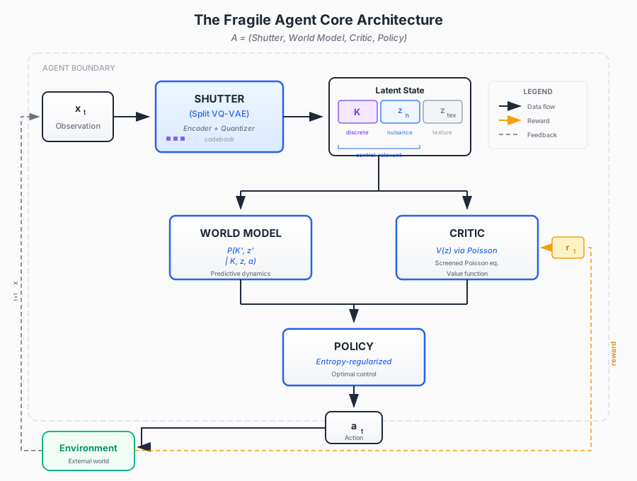
Fig. 1 The Fragile Agent Core Architecture. The agent tuple \(\mathbb{A} = (\text{Shutter}, \text{World Model}, \text{Critic}, \text{Policy})\) showing data flow from observation \(x_t\) through the three-tier latent state \((K, z_n, z_{\mathrm{tex}})\) to action \(a_t\), with environment feedback loop.

The Trinity of Manifolds (Dimensional Alignment)

Now I need to tell you about something that trips up a lot of people, and it’s important enough that I want to be very clear about it.

When we do machine learning, we’re working with three completely different “spaces,” and they must not be confused. It’s like confusing the map with the territory, or confusing the weights in your brain with the things you’re thinking about. These are category errors, and they lead to all sorts of trouble.

Here are the three spaces:

The Physical/Data Space (\(\mathcal{X}\)): This is the raw observation space. Pixels on a screen. Joint angles of a robot. It’s high-dimensional, messy, and full of irrelevant detail. We use Euclidean geometry here because that’s what the hardware gives us.

The Latent/Problem Space (\(\mathcal{Z}\)): This is where the agent actually thinks. It’s the compressed representation that captures what matters for decision-making. And crucially, it has structure—a discrete macro symbol \(K\) for identity, a continuous nuisance coordinate \(z_n\) for pose/position, and a texture channel \(z_{\mathrm{tex}}\) for reconstruction detail.

The Parameter/Model Space (\(\Theta\)): This is the space of neural network weights. It’s where gradient descent lives. And it has its own geometry—the Fisher-Rao geometry that tells you how changing weights affects the distribution of outputs.

To prevent category errors, we formally distinguish three manifolds with distinct geometric structures:

Manifold	Symbol	Coordinates	Metric Tensor	Role
Physical/Data	\(\mathcal{X}\)	\(x \in \mathbb{R}^D\)	\(I\) (Euclidean)	Raw observations—the “hardware”
Latent/Problem	\(\mathcal{Z}=\mathcal{K}\times \mathcal{Z}_{n}\times \mathcal{Z}_{\mathrm{tex}}\)	\((K, z_{n}, z_{\mathrm{tex}})\) with \(K \in \mathcal{K}\), \(z_{n}\in\mathbb{R}^{d_n}\), \(z_{\mathrm{tex}}\in\mathbb{R}^{d_{\mathrm{tex}}}\)	\(d_{\mathcal{K}} \oplus G_{n}(z_{n};K)\)	Symbolic macro-register + structured nuisance coordinates + reconstruction-only texture
Parameter/Model	\(\Theta\)	\(\theta \in \mathbb{R}^P\)	\(\mathcal{F}(\theta)\) (Fisher-Rao)	Configuration space—the “weights”

Dimensional Verification:

• The shutter \(E: \mathcal{X} \to \mathcal{K}\times \mathcal{Z}_n\times \mathcal{Z}_{\mathrm{tex}}\) is a contraction in structured continuous degrees of freedom (\(d_n \ll D\)) plus a finite-rate quantization in the macro channel (\(\log|\mathcal{K}|\) nats); texture may remain high-rate but is firewall-restricted to reconstruction/likelihood.

• The policy \(\pi_\theta\) is typically a map on macrostates (or their code embeddings) \(\pi_\theta:\mathcal{K}\to\mathcal{A}\). If a structured nuisance coordinate \(z_n\) is required for actuation, treat it as an explicit typed input (policy on \((K,z_n)\)) and keep enclosure/closure defined at the macro layer (Conditional Independence and Sufficiency (Causal Enclosure)). By contrast, dependence on texture \(z_{\mathrm{tex}}\) is a causal leak for control and should be prohibited by architecture and monitored (texture is reconstruction-only).

• The metric \(G_{n}\) is defined on the structured nuisance coordinates \(\mathcal{Z}_n\) (and/or the induced geometry of the codebook embedding), not on \(\Theta\); texture is excluded from the control metric.

The Anti-Mixing Principle

Never conflate \(\mathcal{F}(\theta)\) (parameter-space Fisher) with \(G(z)\) (state-space metric). They live on different manifolds and measure different quantities:

• \(\mathcal{F}(\theta)\): How the policy changes with weights (used by TRPO/PPO)

• \(G_n(z_n;K)\): How the policy changes with structured nuisance coordinates (used by the Fragile Agent)

This is like confusing how your neurons fire with what you’re thinking about. They’re related, but they’re not the same thing.

Remark (WFR Foundation). The product metric \(d_{\mathcal{K}} \oplus G_n\) is a first approximation treating discrete and continuous components separately. Wasserstein-Fisher-Rao Geometry: Unified Transport on Hybrid State Spaces provides the rigorous Wasserstein-Fisher-Rao (WFR) metric that unifies these components variationally: transport (Wasserstein) handles continuous motion within charts, while reaction (Fisher-Rao) handles discrete jumps between charts.

The Shutter as a VQ-VAE (Discrete Macro, Continuous Micro)

Now let’s look more carefully at the Shutter—the encoder that compresses observations into the latent space. This is where some really important things happen.

Here’s the problem: if you use a standard autoencoder, everything gets mixed together. The identity of an object, its position, the lighting, the texture of its surface—all of it gets squished into one continuous vector. And that causes trouble, because:

1. You can’t easily count or enumerate states (useful for theory and for tabular methods)

2. Adversarial noise in the texture can fool the policy

3. You waste capacity on details that don’t matter for control

The solution is to split the latent space into channels with different roles. And the key to making one of those channels discrete is something called a Vector Quantized VAE, or VQ-VAE.

The information-theoretic/control interpretation benefits from an explicit discrete latent register: a countable set of macrostates on which we can apply Shannon/algorithmic statements without differential-entropy ambiguities. This is provided by a VQ-VAE macro-encoder.

Researcher Bridge: Adversarial Immunity via Firewalling

Standard Autoencoders mix all information into a single vector, making them vulnerable to “texture” attacks (adversarial noise). We split the latent space into three channels: Discrete Symbols (\(K\)), Nuisance (\(z_n\)), and Texture (\(z_{\mathrm{tex}}\)). By architectural design, the Policy is blind to the Texture channel. This creates a mathematical firewall: the agent uses texture for reconstruction, but is architecturally constrained from making decisions based on non-causal pixel noise.

The Three-Channel Decomposition

Imagine you’re looking at a photograph of a coffee mug on a table. What information is in that image?

First, there’s the identity: it’s a mug, not a bowl or a vase. That’s a discrete thing—you can list all the objects you know about and point to one of them. This goes into the macro channel \(K\).

Second, there’s the pose and position: where is the mug? What angle are we viewing it from? How far away is it? This is continuous and structured—you can parameterize it with a few numbers. This goes into the nuisance channel \(z_n\).

Third, there’s the texture and fine detail: the exact pattern on the mug, the way the light reflects off the glaze, the grain of the wood table. This is needed to reconstruct the image, but it shouldn’t affect your decision about whether to pick up the mug. This goes into the texture channel \(z_{\mathrm{tex}}\).

We factor the latent as:

\[ Z_t := (K_t, z_{n,t}, z_{\mathrm{tex},t}), \qquad K_t \in \mathcal{K}\ \text{(discrete; may be hierarchical)}, \quad z_{n,t}\in\mathbb{R}^{d_n}\ \text{(continuous nuisance; gauge fiber in {ref}`sec-local-gauge-symmetry-nuisance-bundle`)}, \quad z_{\mathrm{tex},t}\in\mathbb{R}^{d_{\mathrm{tex}}}\ \text{(continuous texture)}.\]

For the Attentive Atlas shutter, the macro register is a two-level tuple:

\[ K_t = (K_{\text{chart}}, K_{\text{code}}),\]

with \(K_{\text{chart}}\in\{1,\dots,N_c\}\) and \(K_{\text{code}}\in\{1,\dots,N_v\}\).

How VQ-VAE Makes Discrete Symbols

Here’s the beautiful trick in VQ-VAE. Instead of having a continuous latent vector, you have a codebook—a fixed set of vectors that the encoder can point to.

Think of it like this: instead of describing a color by its exact RGB values (continuous), you describe it by pointing to the closest swatch in a paint store catalog (discrete). You lose some precision, but you gain the ability to count and enumerate your states.

Macro codebook (symbols). Let \(\mathcal{K}=\{1,\dots,|\mathcal{K}|\}\) and let \(\{e_k\}_{k\in\mathcal{K}}\subset\mathbb{R}^{d_m}\) be a learned codebook. Given an observation \(x\) the macro encoder produces a pre-quantized vector \(z_e(x)\in\mathbb{R}^{d_m}\) and the VQ projection chooses the nearest code:

\[ K(x) := \arg\min_{k\in\mathcal{K}} \|z_e(x)-e_k\|_2^2, \qquad z_{\text{macro}}(x):=e_{K(x)}.\]

We equip \(\mathcal{K}\) with the induced finite metric \(d_{\mathcal{K}}(k,k'):=\|e_k-e_{k'}\|_2\) (or its \(G_\mu\)-weighted variant), so \(\mathcal{Z}\) is a bundle of continuous fibres over a discrete base.

Connection to RL #5: Tabular Q-Learning as Degenerate VQ-VAE

The General Law (Fragile Agent): The state is encoded via a learned VQ-VAE discretization:

\[ K(x) := \arg\min_{k \in \mathcal{K}} \|z_e(x) - e_k\|_2^2\]

where \(\{e_k\}_{k \in \mathcal{K}}\) is a learned codebook and \(z_e(x)\) is the encoder output.

The Degenerate Limit: Set \(|\mathcal{K}| = |\mathcal{S}|\) (codebook size equals state space) and encoder \(z_e = \text{identity}\).

The Special Case (Standard RL):

\[ K(x) = s \in \{1, \ldots, N\} \quad \text{(tabular state index)}\]

This recovers Tabular Q-Learning with discrete state enumeration.

Result: Tabular RL is VQ-VAE with a trivial encoder and fixed codebook. MuZero/Dreamer are the limit \(|\mathcal{K}| \to \infty\) (continuous latent, no explicit symbols).

What the generalization offers:

• Learned discretization: codebook adapts to task structure

• Information bottleneck: \(I(X; K) \le H(K) \le \log|\mathcal{K}|\) bounds capacity

• Hybrid: discrete macro-register enables symbolic world models while continuous channels preserve detail

The Attentive Atlas Shutter

Now let me tell you about a more sophisticated version of this, called the Attentive Atlas. The idea is that different parts of your state space might need different codebooks—like having different paint catalogs for different types of surfaces.

Attentive Atlas shutter (TopoEncoder implementation). The shutter in topoencoder.py uses a shared feature extractor \(f(x)\), then:

• Key projection: \(k(x)=W_k f(x)\)

• Value projection: \(v(x)=W_v f(x)\)

• Chart query bank: \(\{q_i\}_{i=1}^{N_c}\)

• Cross-attention routing:

  \[ w_i(x) = \frac{\exp(\langle k(x), q_i\rangle/\sqrt{d})}{\sum_j \exp(\langle k(x), q_j\rangle/\sqrt{d})}, \qquad K_{\text{chart}} = \arg\max_i w_i(x).\]

Each chart has its own codebook \(\{e_{i,c}\}_{c=1}^{N_v}\). For each chart, pick the closest code

\[ K_{\text{code},i}(x) := \arg\min_c \|v(x)-e_{i,c}\|_2^2,\]

then form a soft blended code for differentiability:

\[ z_q(x) := \sum_i w_i(x)\, e_{i,K_{\text{code},i}(x)}.\]

The hard code index used for discrete state is \(K_{\text{code}}:=K_{\text{code},K_{\text{chart}}}(x)\).

The Residual Split: Separating Nuisance from Texture

After quantization, there’s still information left over—the “residual” between what the encoder produced and what the codebook captured. We split this residual into two parts: structured nuisance (things like position that might matter for actuation) and texture (fine details that only matter for reconstruction).

Recursive residual split (TopoEncoder). The shutter then decomposes the value residual:

\[ c_{\mathrm{bar}}(x):=\sum_i w_i(x)c_i,\qquad v_{\mathrm{local}}(x):=v(x)-c_{\mathrm{bar}}(x), \]

\[ K_{\text{code},i}(x):=\arg\min_c\|v_{\mathrm{local}}(x)-e_{i,c}\|_2^2, \qquad z_q(x):=\sum_i w_i(x)e_{i,K_{\text{code},i}(x)}, \]

\[ \Delta_{\text{total}}=v_{\mathrm{local}}-\operatorname{sg}[z_q], \qquad z_n=\text{StructureFilter}(\Delta_{\text{total}}), \qquad z_{\mathrm{tex}}=\Delta_{\text{total}}-z_n.\]

Finally, the geometric latent for the decoder is

\[ z_q^{\text{st}} = v_{\mathrm{local}} + \operatorname{sg}[z_q-v_{\mathrm{local}}], \qquad z_{\text{geo}} = c_{\mathrm{bar}} + z_q^{\text{st}} + z_n,\]

so reconstruction uses the chart center, discrete macro code, structured nuisance, and the separate texture residual at the decoder input.

Making the Macro Channel Invariant to Pose

Here’s a practical problem: if you show the same mug from two different angles, you want the macro symbol \(K\) to be the same (it’s the same mug!), but of course the pixels are completely different. How do we achieve this?

Canonicalization and symmetry quotienting (optional). Let \(G_{\text{spatial}}\) be a nuisance group acting on observations (Symmetries and Gauge Freedoms (Operational)). A practical way to make the macro register invariant to pose/basis choices is to insert a canonicalization map \(C_\psi:\mathcal{X}\to\mathcal{X}\) before quantization and to train it so that

\[ C_\psi(g\cdot x)\approx C_\psi(x)\qquad (g\in G_{\text{spatial}}).\]

One implementation is a Spatial Transformer Network (STN) that predicts and applies an input warp before the VQ encoder [Jaderberg et al., 2015]. An alternative is to use an explicitly group-equivariant encoder and then pool to an invariant statistic [Cohen and Welling, 2016].

Operationally, we replace the quantizer input \(x\) by \(\tilde x:=C_\psi(x)\) and define \(K(x):=K(\tilde x)\). This realizes the quotienting intent “\(K\) represents \(x/G_{\text{spatial}}\)” without requiring an exact quotient construction.

The Design Goal: Identity vs Nuisance vs Texture

Let me summarize what we’re trying to achieve with this three-way split.

Identity vs nuisance vs texture. With canonicalization enabled, the design goal is a three-way separation:

• \(K_t\) captures invariant identity (“what”) needed for prediction and control.

• \(z_{n,t}\) carries structured nuisance (“where/how”, pose/basis/disturbance coordinates) that may be needed for actuation or for explaining boundary-induced deviations, but must remain disentangled from \(K\).

• \(z_{\mathrm{tex},t}\) carries texture/detail needed for reconstruction/likelihood only and is treated as measurement/emission residual: it must not be required for macro closure or for control decisions.

This separation is enforced by orbit-invariance and (macro perpendicular to nuisance/texture) disentanglement losses in Defect Functionals: Implementing Regulation.A and monitored by SymmetryCheck/DisentanglementCheck (Diagnostics: Stability Checks (Monitors)). The jump/residual machinery (Sieve Events as Projections / Reweightings) is attached to \(z_n\) (structured disturbances), not to \(z_{\mathrm{tex}}\).

Remark (Motor Texture Extension). Motor Texture: The Action Residual extends this decomposition to the motor/action side: \(a_t = (K^{\text{act}}_t, z_{n,\text{motor}}, z_{\text{tex,motor}})\). The motor texture \(z_{\text{tex,motor}}\) (tremor, fine motor noise) is constrained by the Motor Texture Firewall; the symplectic duality is stated in Motor Texture: The Action Residual. The Dual Atlas Architecture defines a Dual Atlas Architecture where \(\mathcal{A}_{\text{vis}}\) (visual) and \(\mathcal{A}_{\text{act}}\) (action) are related by Legendre transform.

Connection to RL #6: Options Framework as Read-Only Codebook

The General Law (Fragile Agent): The agent’s state is a Split VQ-VAE with learned hierarchy:

\[ Z_t = (K_t, z_{n,t}, z_{\mathrm{tex},t}) \in \mathcal{K} \times \mathcal{Z}_n \times \mathcal{Z}_{\mathrm{tex}}\]

where:

• \(K_t \in \mathcal{K}\): Discrete macro-symbol (learned via codebook)

• \(z_{n,t}\): Continuous structured nuisance

• \(z_{\mathrm{tex},t}\): Texture residual (reconstruction-only)

The Shutter forces temporal decoupling: \(K\) evolves slowly, \((z_n, z_{\mathrm{tex}})\) evolve fast.

The Degenerate Limit: Hard-code the semantics of \(K\) to be fixed sub-policies rather than learned symbols.

The Special Case (Standard RL):

\[ \text{Options Framework (Sutton et al.)}: o \in \{o_1, \ldots, o_N\}, \quad \pi_o(a|s)\]

where \(o\) is a fixed option index and \(\pi_o\) is a pre-specified intra-option policy.

Result: Standard HRL is the Fragile Agent with a read-only codebook. The Option index \(o\) becomes our macro \(K\); the “intra-option state” becomes our texture.

What the generalization offers:

• Learned hierarchy: codebook adapts to task, not hand-designed

• Temporal shutter: macro evolves on natural timescale, not fixed option duration

• Nuisance channel: explicitly models “how” (pose/disturbance) separate from “what” (identity)

The Continuous Channels: Nuisance and Texture

While the macro channel \(K\) is discrete, the nuisance and texture channels remain continuous. They’re modeled with Gaussian posteriors, but with different roles.

Nuisance residual (\(z_n\)). The nuisance channel remains continuous, e.g. with a Gaussian posterior

\[ q_\phi(z_n\mid x)=\mathcal{N}(\mu_\phi(x),\operatorname{diag}(\sigma_\phi^2(x))),\]

with a task-appropriate prior \(p(z_n)\) (often standard normal as a conservative default). The key requirement is typed: nuisance may influence reconstruction and may be used to explain structured deviations, but macro prediction/closure must not require it beyond \((K_t,K^{\text{act}}_t)\) (Conditional Independence and Sufficiency (Causal Enclosure)).

Texture residual (\(z_{\mathrm{tex}}\)). Texture is modeled as a separate continuous residual with posterior

\[ q_\phi(z_{\mathrm{tex}}\mid x)=\mathcal{N}(\mu_{\mathrm{tex}}(x),\operatorname{diag}(\sigma_{\mathrm{tex}}^2(x))),\]

and a simple high-entropy prior \(p(z_{\mathrm{tex}})=\mathcal{N}(0,I)\) so that matching \(q_\phi(\cdot\mid x)\) to \(p\) operationalizes the statement “texture is reconstruction-only”: it should explain details that do not belong in the macro dynamics.

The Training Objective

Now, how do we train this whole thing? We need an objective that encourages:

1. Good reconstruction (the decoder should reproduce the input)

2. Codebook learning (the codes should cover the data distribution)

3. Commitment (the encoder should commit to nearby codes)

4. Proper regularization of the continuous channels

VQ-VAE objective (with nuisance + texture). With a decoder \(p_\theta(x\mid z_{\text{macro}},z_n,z_{\mathrm{tex}})\) and stop-gradient operator \(\operatorname{sg}[\cdot]\), the canonical loss is

\[\begin{split} \begin{aligned} \mathcal{L}_{\text{shutter}} &= \mathbb{E}\Big[-\log p_\theta(X\mid e_{K(X)}, Z_n, Z_{\mathrm{tex}})\Big] \\[4pt] &\quad + \underbrace{\lVert \operatorname{sg}[z_e]-e_{K}\rVert_2^2}_{\text{codebook}} + \underbrace{\beta\lVert z_e-\operatorname{sg}[e_K]\rVert_2^2}_{\text{commit}} \\[4pt] &\quad + \underbrace{\beta_n D_{\mathrm{KL}}(q_\phi(Z_n\mid X)\Vert p(Z_n))}_{\text{nuisance prior}} \\[4pt] &\quad + \underbrace{\beta_{\mathrm{tex}} D_{\mathrm{KL}}(q_\phi(Z_{\mathrm{tex}}\mid X)\Vert p(Z_{\mathrm{tex}}))}_{\text{texture-as-residual}} \end{aligned}\end{split}\]

Units: \(\beta\), \(\beta_n\), and \(\beta_{\mathrm{tex}}\) are dimensionless weights; each \(D_{\mathrm{KL}}\) is measured in nats. In the Attentive Atlas shutter, the codebook/commitment terms are computed per chart and weighted by \(w_i(x)\) so inactive charts do not receive spurious updates.

Why Discretization Matters: Information-Theoretic Bounds

Here’s the beautiful thing about having a discrete macro channel: we can make exact information-theoretic statements. None of the fuzziness of differential entropy—just good old Shannon theory.

Information-theoretic capacity becomes explicit. Because \(K\) is discrete,

\[ I(X;K)\le H(K)\le \log|\mathcal{K}|.\]

For the hierarchical macro \((K_{\text{chart}},K_{\text{code}})\), this becomes \(H(K)\le \log(N_c N_v)\). For deterministic nearest-neighbor quantization, \(H(K\mid X)=0\) and hence \(I(X;K)=H(K)\): the macro channel is a bounded-rate symbolic memory with capacity at most \(\log|\mathcal{K}|\) nats.

This is profound. It means we have a hard limit on how much information can flow through the macro channel, and we can monitor it. If the agent is using too much or too little of its capacity, we can see it and fix it.

Connection to RL #10: Soft Actor-Critic as Degenerate MaxEnt Control

The General Law (Fragile Agent): The agent optimizes an entropy-regularized objective on the Riemannian manifold \((\mathcal{Z}, G)\):

\[ \mathcal{F}[p, \pi] = \int_{\mathcal{Z}} p(z) \Big( V(z) - T_c\, H(\pi(\cdot|z)) \Big) d\mu_G\]

where \(d\mu_G = \sqrt{|G|}\, dz\) is the Riemannian volume form and \(T_c\) is the entropy weight (cognitive temperature).

The Degenerate Limit: Restrict entropy regularization to action space only; ignore state-space geometry (\(G \to I\)).

The Special Case (Standard RL):

\[ J_{\text{SAC}}(\pi) = \mathbb{E}\left[\sum_{t=0}^\infty \gamma^t \big(r_t + \alpha H(\pi(\cdot|s_t))\big)\right]\]

This recovers Soft Actor-Critic (SAC) with action entropy bonus.

Result: SAC is MaxEnt control on a flat manifold with entropy only in action space. The Fragile Agent extends this to: (1) entropy in representation space via VQ commitment, (2) geometry-aware updates via \(G\), and (3) capacity constraints via the codebook.

What the generalization offers:

• Representation entropy: VQ commitment \(\beta\|z_e - \text{sg}[e_K]\|^2\) prevents collapse

• State-space geometry: under the stated calibration ansatz, one-step covariance \(\Sigma_{\mathrm{step}}(z) \propto T_c\,G^{-1}(z)\) adapts to local sensitivity

• Capacity bound: \(H(K) \le \log|\mathcal{K}|\) provides hard information constraint

Rate-Distortion: The Information-Theoretic Foundation

For those who want the deep foundation: VQ-VAE is really a computational instantiation of rate-distortion theory—the fundamental trade-off between compression and fidelity.

Rate-distortion / MDL viewpoint (optional but canonical). Because \(K\) is a discrete string, an explicit entropy model \(p_\psi(K)\) defines a literal expected codelength \(\mathbb{E}[-\log p_\psi(K)]\) (in nats). Adding this term yields the Lagrangian form of lossy source coding:

\[ \min_{E,D}\ \mathbb{E}\big[d(X,\hat{X})\big] + \lambda_{\text{RD}}\,\mathbb{E}\big[-\log p_\psi(K)\big],\]

with rate controlled by the symbolic model and distortion controlled by the decoder. This is the rigorous information-theoretic envelope in which VQ-VAE-style macrostates live. Units: \(\lambda_{\text{RD}}\) has units of the distortion scale divided by nats (dimensionless if \(d\) is itself a negative-log-likelihood in nats).

Notation note (micro split). Earlier sections (and some later, legacy blocks) use \(z_\mu\) / \(\mathcal{Z}_\mu\) to denote “the continuous micro channel”. In the refined typed specification, this channel is split as

\[ z_\mu \equiv (z_n, z_{\mathrm{tex}}),\]

where \(z_n\) is structured nuisance (may be used for actuation/auditing) and \(z_{\mathrm{tex}}\) is texture (likelihood/reconstruction-only). Unless a section explicitly discusses texture, occurrences of \(z_\mu\) should be read as the nuisance channel \(z_n\).

Why All This Structure Matters

Let me step back and explain why we’ve gone to all this trouble.

Metatheorems unlocked by discretization.

• A discrete macro-register makes coding-theoretic and finite-memory update bounds applicable.

• Macro-trajectories become literal strings \(K_{0:T}\), so Levin/Kolmogorov-style horizon arguments become well-typed (see the Levin-Search metatheorem in Appendix A: Full Derivations (Capacity-Constrained Curvature Functional)).

In other words: by making part of our representation discrete, we’ve made the theory work. We can prove things. We can bound things. We can monitor things. That’s the payoff for all this structure.

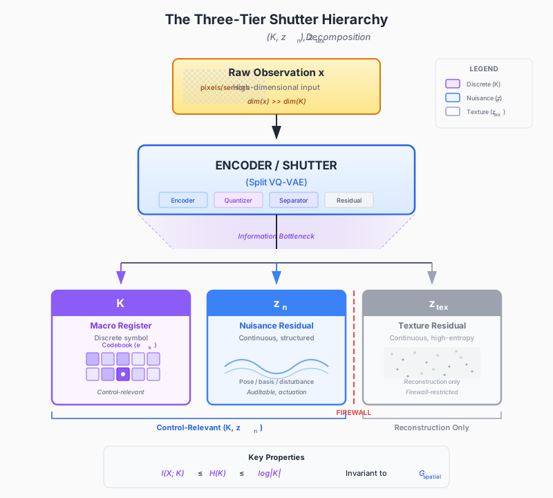
Fig. 2 The Three-Tier Shutter Hierarchy. The VQ-VAE shutter decomposes observations into three channels: \(K\) (discrete macro-register, control-relevant), \(z_n\) (continuous nuisance, structured), and \(z_{\mathrm{tex}}\) (texture, reconstruction-only). The information bottleneck at quantization ensures \(I(X; K) \le H(K) \le \log|\mathcal{K}|\).

The Bridge: RL as Lyapunov-Constrained Control (Neural Lyapunov Geometry)

Now we come to something that I think is really important—the connection between reinforcement learning and control theory. These two fields have developed largely independently, but they’re really talking about the same thing from different angles.

Standard Reinforcement Learning maximizes expected return. That’s the optimization view: find the policy that gets the most reward.

Robust control enforces stability by requiring a Lyapunov-like decrease condition. That’s the safety view: make sure the system doesn’t blow up.

Here’s the insight: these perspectives align around the same mathematical objects. The value function that RL tries to maximize is the same thing as the Lyapunov function that control theory uses to prove stability. If we’re smart, we can get both optimization and stability from the same object.

Perspective	Objective	Mechanism
Optimization	Minimize expected cost-to-go \(V(z)\)	Gradient-based policy/value updates
Control Theory	Ensure stability: \(\dot{V}(z) \le -\lambda_{\text{Lyap}} V(z)\), \([\lambda_{\text{Lyap}}]=s^{-1}\)	Lyapunov constraint
Reinforcement Learning	Improve value estimates/policy	TD learning + policy gradients

The key insight is that these perspectives align around the same mathematical objects: a scalar value/cost-to-go function (for the exact component of the cost 1-form, with reward convention via \(\mathcal{C}=-\mathcal{R}\)) and constraints on how fast it can improve without destabilizing the loop.

Connection to RL #18: Lyapunov Stability as Implicit Hope

The General Law (Fragile Agent): After choosing the terminal/baseline normalization so that the Lyapunov candidate \(\widetilde V:=V-V_{\mathrm{eq}}\ge0\), the critic serves as a Control Lyapunov Function with explicit stability constraint:

\[ \dot{\widetilde V}(z) := \nabla_A \widetilde V(z)^\top \dot{z} \le -\lambda_{\text{Lyap}} \widetilde V(z), \quad [\lambda_{\text{Lyap}}] = s^{-1}\]

The Sieve (Node 7: StiffnessCheck) monitors the local gradient norm against a declared threshold \(\|\nabla_A V\| > \epsilon\) on the sampled operating region; it is not a global lower-bound theorem. Bifurcation is monitored separately (Node 7a).

The Degenerate Limit: Remove the explicit stability check. Assume SGD will find a stable fixpoint.

The Special Case (Standard RL): Standard policy gradient methods (PPO, SAC, etc.) optimize \(\mathbb{E}[R]\) without enforcing \(\dot{V} \le -\lambda_{\text{Lyap}} V\). Stability is an implicit hope, not a guarantee.

Result: Standard RL oscillates and diverges precisely because it tries to find a Lyapunov function without enforcing the Lyapunov conditions. The Fragile Agent makes stability a hard constraint, not an emergent property.

What the generalization offers:

• Explicit stability: \(\dot{V} \le -\lambda_{\text{Lyap}} V\) is enforced, not hoped for

• Bifurcation detection: Node 7a monitors \(\det(J)\) for approaching instabilities

• Remediation: violations trigger conservative updates, not catastrophic divergence

A Geometry-Regularized Objective (Natural-Gradient View)

Here’s a question that’s going to lead us somewhere important: when you update a policy, how big a step should you take?

The naive answer is “as big as possible without things breaking.” But what does “breaking” mean? And how do you measure “big”?

The key insight is that “size” depends on where you are. Imagine you’re walking on a mountainside. A step of one meter means something very different depending on whether you’re on a gentle slope or the edge of a cliff. The same step that’s perfectly safe in one place might kill you in another.

The same thing is true in learning. A policy update of a certain size might be fine when the value function is flat, but catastrophic when the value function is sharply curved. We need a notion of distance that adapts to the local geometry.

Throughout this section, the geometry and action functional live on the latent state manifold \(\mathcal{Z}\): the updates are trajectories \(z(t)\) induced by the policy and dynamics. Parameter updates in \(\Theta\) are separate; any comparison to \(\theta\) updates is an explicit analogy that conflates \(\mathcal{Z}\) and \(\Theta\) (the category error in Section 2.6).

We can write an update objective that combines (i) a geometry-aware smoothness/trust-region penalty and (ii) a value-improvement term:

\[ \mathcal{S} = \int \left( \underbrace{\frac{1}{2} \lVert\dot{z}\rVert^2_{G}}_{\text{Update smoothness / trust region}} - \underbrace{V(z)}_{\text{cost potential}} \right) dt\]

Where \(\lVert\cdot\rVert_G\) is the norm under a state-space sensitivity metric \(G\) (Second-Order Sensitivity: Value Defines a Local Metric). This biases updates toward paths that are conservative in sensitive regions and more aggressive where the value landscape is well-conditioned.

Connection to RL #2: SGD as Degenerate Geodesic Flow

The General Law (Fragile Agent): State updates follow geodesic flow on the Riemannian manifold \((\mathcal{Z}, G)\):

\[ \mathcal{S} = \int \left( \frac{1}{2} \|\dot{z}\|_G^2 - V(z) \right) dt\]

The Euler–Lagrange equations yield a forced geodesic equation with cost force \(-G^{-1}dV\); when the potential is constant this reduces to geodesic flow. The term \(-dV/dt\) would be a boundary term and cannot supply this force.

The Degenerate Limit: Set \(G = I\) (flat metric). Geodesics become straight lines in state space.

The Special Case (Standard RL):

\[ \theta_{t+1} = \theta_t + \eta \nabla_\theta J(\theta)\]

If one conflates state space with parameter space (the category error in Section 2.6), this recovers Euclidean SGD—parameter updates as straight-line steps in flat space.

Result: SGD ignores curvature. In ill-conditioned regions (sharp valleys, saddles), this leads to oscillation, slow convergence, or divergence. Geodesic flow automatically adapts step size to local geometry.

What the generalization offers:

• Automatic preconditioning: ill-conditioned directions are damped

• Coordinate invariance: behavior doesn’t depend on arbitrary parameterization

• Interpretation: updates correspond to stationary paths of the action functional on the value landscape

Comparison: Euclidean vs Geometry-Aware Updates

Aspect	Euclidean (parameter-space view)	Geometry-aware (state-space flow)
Metric	\(\lVert\cdot\rVert_2\) (flat)	\(\lVert\cdot\rVert_G\) (curved)
Step Size	Constant everywhere	Varies with curvature
Near ill-conditioned regions	Large steps cause instability	Small steps ensure safety
In Valleys	Same as cliffs	Large steps ensure efficiency
Failure Mode	BarrierBode (oscillation)	Prevented by geometry

Second-Order Sensitivity: Value Defines a Local Metric

Now let’s get concrete about what this metric \(G\) actually is.

In information geometry and second-order optimization, a local metric captures how sensitive the objective and the policy are to changes in state coordinates [Amari, 1998]. For the Fragile Agent, we define a state-space sensitivity metric \(G_{ij}\) that combines value curvature with control sensitivity in the latent state.

The intuition is this: if you’re in a region where the value function is sharply curved, then small changes in state lead to big changes in value. That’s a dangerous place to be aggressive. Conversely, if the value function is flat, you can afford to take bigger steps.

Researcher Bridge: Beyond Parameter-Space Adam

Standard optimizers like Adam or K-FAC use the Fisher Information of the Parameter Manifold (\(\Theta\)) to scale updates. This ignores the geometry of the environment. The Fragile Agent introduces a metric \(G\) on the Latent State Manifold (\(\mathcal{Z}\)). Why this matters: It acts as a state-dependent preconditioner. In high-risk or high-sensitivity regions (sharp value gradients), the eigenvalues of \(G\) increase, automatically forcing the agent to take smaller, more cautious steps. This transforms natural-gradient updates from a weight-update technique into a coordinate-invariant update rule.

Definition 5 (State-Space Sensitivity Metric)

The value-curvature component of the state-space sensitivity metric at a point \(z\) in the latent space is defined from the symmetric Hessian of the value function, with a PSD proxy used when enforcing metric positivity:

\[ (G_V)_{ij} = \frac{\partial^2 V}{\partial z_i \partial z_j} \quad \text{(theory)}, \qquad (G_V)_{ij} \approx c_V\,\frac{\partial V}{\partial z_i}\frac{\partial V}{\partial z_j} \quad \text{(Gauss--Newton proxy)}.\]

The complete metric used elsewhere is \(G = G_V + \lambda_G G_\pi\) with \(G_\pi\) the state-space Fisher component (Definition Definition 6). Units: \([(G_V)_{ij}]=\mathrm{nat}\,[z]^{-2}\) if \(z\) is measured in units \([z]\); in the proxy form, \(c_V\) carries units \(\mathrm{nat}^{-1}\).

Behavior in Different Regions:

• Flat Region (\(G \approx \text{const}\)): The value curvature is small and the Fisher component is approximately constant (e.g., whitened to \(I\)), so distances are effectively Euclidean up to a fixed scale.

• Curved Region (\(G \gg I\)): The value function is sharply curved (ill-conditioned). The metric rescales distances: a small Euclidean step can correspond to a large change in value/sensitivity.

The Upgrade: From Gradient Descent to Geodesic Flow

This is an analogy across spaces: the left column is a parameter-space update, while the right column is a latent state-space flow governed by \(G\).

Standard RL (parameter space)	State-space Riemannian update
\(\theta \leftarrow \theta + \eta \nabla_\theta \mathcal{L}\)	\(z \leftarrow z - \eta G^{-1}(z)\nabla_z \mathcal{L}\)
Euclidean gradient	State-space natural gradient (Amari)
Ignores curvature	Respects curvature

Connection to RL #1: REINFORCE as Degenerate Natural Gradient

The General Law (Fragile Agent): Latent-state updates (policy-induced trajectories) follow a flow on the Riemannian manifold \((\mathcal{Z}, G)\):

\[ \delta z = -G^{-1}(z) \nabla_z \mathcal{L}\]

where \(G(z)\) is the state-space sensitivity metric (Definition Definition 6).

The Degenerate Limit: Set \(G = I\) (identity matrix). The manifold becomes flat Euclidean space.

The Special Case (Standard RL):

\[ \delta\theta = \nabla_\theta J(\theta) \quad \text{(REINFORCE / Vanilla Policy Gradient)}\]

This recovers REINFORCE with Euclidean gradient ascent.

Result: TRPO/PPO are partial steps toward the general framework—they approximate \(G\) with the parameter-space Fisher Information \(\mathcal{F}(\theta)\), but lack the state-space metric derived from capacity constraints (Theorem Theorem 6).

What the generalization offers:

• Coordinate invariance: updates don’t depend on arbitrary parameterization

• Automatic damping: high-curvature regions (\(G\) large) are updated cautiously

• State-space grounding: metric captures value sensitivity, not just policy sensitivity

In the Fragile Agent implementation, the Riemannian metric lives in state space, not parameter space. The covariant derivative uses a diagonal inverse metric \(M^{-1}(z)\) to scale \(\dot{V}\):

\[ \dot V:=dV(\dot z)=\partial_iV\,\dot z^i.\]

When the update is \(\dot z=-M^{-1}d_AV\), the associated preconditioned descent rate is \(-\lVert d_AV\rVert^2_{M^{-1}}\). The discrete-time estimate \(\Delta z / \Delta t\) supplies \(\dot z\) in practice. Current state-space metric options (diagonal approximations):

• Observation variance (whitening):

  \[ M^{-1}_{ii}(z) = \frac{1}{\mathrm{Var}(z_i) + \epsilon}\]

• Policy Fisher on states:

  \[ M^{-1}_{ii}(z) = \frac{1}{\mathbb{E}[(\partial_{z_i}\log \pi(a|z))^2] + \epsilon}\]

• Gradient RMS (critic):

  \[ M^{-1}_{ii}(z) = \frac{1}{\sqrt{\mathbb{E}[(\partial_{z_i} V)^2]} + \epsilon}\]

In all three cases, \(\epsilon\) is a numerical stabilizer with the same units as the denominator term it is added to.

Important: Parameter-space statistics (e.g., Adam’s \(\hat{v}_t\)) are not used for \(M^{-1}(z)\). They belong to optimizer diagnostics, not state-space geometry.

This is a state-space preconditioning effect: directions with large local sensitivity (large \(G\)) are damped via \(G^{-1}\), while flatter directions are amplified. This is the same qualitative idea as natural-gradient and second-order preconditioning, but applied to latent-state coordinates rather than to parameters [Amari, 1998, Martens and Grosse, 2015].

• High curvature / high sensitivity: \(G\) is large, so \(G^{-1}\) is small. The update slows down automatically.

• Low curvature / low sensitivity: \(G\) is small, so \(G^{-1}\) is large. The update accelerates in well-conditioned regions.

A Practical Diagonal Sensitivity Metric

For practical implementation, we often use a diagonal approximation to the full metric.

A Practical Diagonal Sensitivity Metric:

The four scaling coefficients from Scaling Coefficients: Characterizing the Agent are scalar summaries used by the update scheduler, not entries of the state-space tensor \(G\):

\[ (\alpha, \beta_{\pi}, \gamma_{\text{wm}}, \delta)\]

Where:

• \(\alpha\): critic curvature scale (value landscape sensitivity).

• \(\beta_{\pi}\): policy stochasticity / exploration scale.

• \(\gamma_{\text{wm}}\): world-model volatility / non-stationarity scale.

• \(\delta\): representation drift / codebook stability scale.

These coefficients summarize relative update scales across subsystems and serve as a compact diagnostic for stability monitoring.

The Complete State-Space Metric

For the full picture, we combine the Hessian of the value function with the Fisher information of the policy (how sensitive the policy is to state changes).

Definition 6 (Complete Latent Space Metric)

The complete state-space sensitivity metric on \(\mathcal{Z}\) is defined as:

\[ G_{ij}(z) = \underbrace{(G_V)_{ij}(z)}_{\text{Hessian (value curvature)}} + \lambda_G \underbrace{(G_\pi)_{ij}(z)}_{\text{Fisher (control sensitivity)}}, \qquad (G_\pi)_{ij}(z) := \mathbb{E}_{a \sim \pi} \left[ \frac{\partial \log \pi(a|z)}{\partial z_i} \frac{\partial \log \pi(a|z)}{\partial z_j} \right].\]

Units follow the book’s tracked-nat convention: if log-probabilities carry the tracked unit, then \([G_\pi]=\mathrm{nat}^2[z]^{-2}\) and \([\lambda_G]=\mathrm{nat}^{-1}\) so that \(\lambda_GG_\pi\) has units \(\mathrm{nat}[z]^{-2}\) like \(G_V\). If log-probabilities are treated as dimensionless, the corresponding nat factors are omitted consistently from both terms.

Dimensional Verification:

• \(V\) is a scalar potential (0-form) for the exact component of the cost 1-form on \(\mathcal{Z}\) (reward convention via \(\mathcal{C}=-\mathcal{R}\))

• \(\nabla_z V\) is a 1-form (covector): \(dV = (\partial_i V) dz^i\)

• \(\text{Hess}_z(V) = \partial_i \partial_j V\) is a \((0,2)\)-tensor

• The Fisher term is the covariance of the score function \(\nabla_z \log \pi\), also a \((0,2)\)-tensor

• Requirement (Assumption 2): \(G\) must be a positive-definite \((0,2)\)-tensor. In computation this is enforced by the damped inverse \((\widehat G+\epsilon_t I)^{-1}\).

Operational Interpretation:

• High \(G_{ii}\) (large Hessian or Fisher): the objective/policy is highly sensitive to coordinate \(i\) (ill-conditioned or highly controllable direction)

• Low \(G_{ii}\): weak sensitivity or ignored coordinate \(i\) (flat direction / potential blind spot)

Levi-Civita Connection and Parallel Transport (Optional)

Now, if you really want to understand the geometry, there’s one more piece: how do you move vectors around on a curved space?

On a flat space, this is trivial—you just slide the vector over. But on a curved space, what does “the same direction” even mean at two different points? This is where the Levi-Civita connection comes in.

Because \(G\) is a Riemannian metric on \(\mathcal{Z}\), it induces a unique torsion-free, metric-compatible connection (the Levi-Civita connection). In local coordinates the Christoffel symbols are

\[ \Gamma^k_{ij}(z) = \frac12\,G^{k\ell}(z)\left(\partial_i G_{j\ell}(z)+\partial_j G_{i\ell}(z)-\partial_\ell G_{ij}(z)\right).\]

The covariant derivative of a vector field \(v\) is then

\[ (\nabla_i v)^k = \partial_i v^k + \Gamma^k_{ij}v^j.\]

Why this matters here. Most of the document uses \(G\) operationally via diagonal preconditioning \(G^{-1}\) (which is computationally cheap). The connection becomes relevant when we ask whether updates are path dependent in state space: transporting a tangent vector (e.g., a value gradient direction) around a loop can return a different direction if curvature is present. Diagnostics: Stability Checks (Monitors) introduces an operational HolonomyCheck that detects loop drift without explicitly computing \(\Gamma\).

Physics Isomorphism: Levi-Civita Connection

In Physics: The Levi-Civita connection is the unique torsion-free, metric-compatible connection on a Riemannian manifold. It defines parallel transport and geodesics. The Christoffel symbols \(\Gamma^k_{ij} = \frac{1}{2}G^{kl}(\partial_i G_{jl} + \partial_j G_{il} - \partial_l G_{ij})\) encode how vectors rotate under infinitesimal displacement [do Carmo, 1992].

In Implementation: The latent metric \(G\) induces a Levi-Civita connection with Christoffel symbols (Levi-Civita Connection and Parallel Transport (Optional)):

\[ \Gamma^k_{ij}(z) = \frac{1}{2}G^{kl}(z)\left(\partial_i G_{jl} + \partial_j G_{il} - \partial_l G_{ij}\right)\]

appearing in the geodesic correction term of the dynamics (Definition Definition 69).

Correspondence Table:

Differential Geometry	Agent (Latent Dynamics)
Christoffel symbols \(\Gamma^k_{ij}\)	Geodesic correction in SDE
Parallel transport	Value gradient propagation
Geodesic equation \(\ddot{z}^k + \Gamma^k_{ij}\dot{z}^i\dot{z}^j = 0\)	Free motion under metric
Metric compatibility \(\nabla G = 0\)	Consistent distance measurement
Torsion-free	Symmetric policy gradients

Effect: The Christoffel terms ensure that state updates respect the curved geometry—updates are coordinate-invariant, not Euclidean.

The Metric Hierarchy: Fixing the Category Error

Let me now be very precise about something that causes enormous confusion in the field. There are at least three different “metrics” people talk about in geometric RL, and they are NOT the same thing. Mixing them up is a category error.

A common mistake in geometric RL is conflating three distinct geometries:

Geometry	Manifold	Metric	Lives On	Used By
Euclidean	Parameter Space \(\Theta\)	\(\lVert\cdot\rVert_2\) (flat)	Neural network weights	Adam, SGD
Fisher-Rao	Policy Space \(\mathcal{P}\)	\(F_{\theta\theta} = \mathbb{E}[(\nabla_\theta \log \pi)^2]\)	Policy parameters	TRPO, PPO
State-Space Sensitivity	State Space \(Z\)	\(G_{zz} = \lambda_G\,\mathbb{E}[(\nabla_z \log \pi)^2] + \text{Hess}_z(V)\)	Latent states	Fragile Agent

The Category Error: Using Adam’s \(v_t\) (which approximates \(F_{\theta\theta}\) in Parameter Space) as if it were \(G_{zz}\) (State Space) mixes two different manifolds. This breaks coordinate invariance.

Think of it this way: the parameter space is like the DNA that encodes an organism, while the state space is like the organism’s actual body moving through the world. They’re related—the DNA determines the body—but they’re not the same thing, and you can’t use rules that apply to one directly on the other.

The State-Space Fisher Information:

\[ G_{\pi,ij}(z) = \mathbb{E}_{a \sim \pi} \left[ \frac{\partial \log \pi(a|z)}{\partial z_i} \frac{\partial \log \pi(a|z)}{\partial z_j} \right]\]

This measures the Information Bottleneck between the Shutter (Split VQ-VAE) and the Actuator (Policy):

• High \(G_{\pi,ii}\): The policy is sensitive to state dimension \(i\), meaning high control authority

• Low \(G_{\pi,ii}\): The policy ignores dimension \(i\), indicating a potential blind spot

Why This Matters:

• Coordinate Invariance: The agent’s behavior is invariant to how you encode \(z\)

• Natural-Gradient Paths: updates follow shortest/least-distorting paths under the chosen metric

• Stability: the metric discourages overly large updates in regions where the model/value is highly sensitive

The Covariant Regulator uses the State-Space Fisher Information \(G_\pi\) (or its diagonal) to scale update magnitudes. While standard RL uses Fisher in Parameter Space (TRPO/PPO), the Fragile Agent uses Fisher in State Space to stabilize Causal Induction.

Connection to RL #3: TRPO/PPO as Degenerate WFR Trust Region

The General Law (Fragile Agent): Define the state-space sensitivity metric \(G(z)\):

\[ G_{ij}(z) = \lambda_G\,\mathbb{E}_{a \sim \pi}\left[\frac{\partial \log\pi(a|z)}{\partial z_i} \frac{\partial \log\pi(a|z)}{\partial z_j}\right] + \nabla^2_z V(z)\]

The trust region is a belief-space ball under the Wasserstein-Fisher-Rao distance (Definition Definition 53, Wasserstein-Fisher-Rao Geometry: Unified Transport on Hybrid State Spaces):

\[ d_{\mathrm{WFR}}(p_{\text{new}}, p_{\text{old}}) \le \epsilon\]

Quadratic proxy (one-step WFR action): for a small update over \(\Delta s\) with predicted transport/reaction \((v, r_{\text{WFR}})\) and baseline belief density \(p_{\text{old}}\), approximate

\[ d_{\mathrm{WFR}}^2(p_{\text{new}}, p_{\text{old}}) \approx (\Delta s)^2 \int_{\mathcal{Z}} \left(\|v\|_G^2 + \lambda_{\text{WFR}}^2 |r_{\text{WFR}}|^2\right) p_{\text{old}}\, d\mu_G\]

Here \(\lambda_{\text{WFR}}\) is the WFR transport/reaction length scale (Definition Definition 53), and \(r_{\text{WFR}}\) is the WFR reaction rate from the unbalanced continuity equation. This approximation is written in the conservative/gauge-fixed case (otherwise include the \(-2\langle A, v\rangle\) term from the WFR action). In practice, one can use cheaper proxies (diagonal/local quadratic WFR, or entropic/sliced approximations) that retain the transport+reaction structure while avoiding a full transport solve.

The Degenerate Limit: Replace the belief-space WFR constraint with a parameter-space KL/Fisher trust region, discarding state geometry.

The Special Case (Standard RL):

\[\begin{split} \text{TRPO: } D_{\text{KL}}(\pi_\theta \| \pi_{\theta'}) \le \delta \quad \text{(parameter-space constraint)} \\ \text{PPO: } \text{clip}(\rho, 1-\epsilon, 1+\epsilon) \quad \text{(surrogate approximation)}\end{split}\]

Result: TRPO/PPO constrain updates in the wrong space. They measure “how much the policy changed” but not the belief transport/reaction distance in state space.

What the generalization offers:

• Correct manifold: state-space metric \(G(z)\) captures value sensitivity, not just policy sensitivity

• Coordinate invariance: behavior independent of neural network parameterization

• Semantic trust region: constraint based on belief transport/reaction distance, not just the policy distribution

The HJB Correspondence (Costs as Value Updates)

Now we come to the central equation of optimal control: the Hamilton-Jacobi-Bellman equation. This is the continuous-time, rigorous version of what you might know as the Bellman equation from RL textbooks.

The idea is beautiful: there’s a consistency condition that any optimal value function must satisfy. At every point in state space, the rate of change of the value function along an optimal trajectory must balance with the instantaneous cost and control effort.

We replace the heuristic Bellman equation [Bellman, 1957] with the rigorous Hamilton-Jacobi-Bellman (HJB) Equation:

\[ \lambda V(z)=\min_a\left[\mathcal{C}_i(z)f^i(z,a)+\mathfrak{D}(z,a)+\mathcal{L}_{f(\cdot,a)}V(z)\right]\quad(+\,T_c\Delta_GV), \qquad \lambda=-\frac{\ln\gamma}{\Delta t}. \]

Here \(\mathcal{C}\) is the cost 1-form; in a reward convention set \(\mathcal{C}:=-\mathcal{R}\). The exact component of \(\mathcal{C}\) defines the cost-to-go \(V=-\Phi\) (up to a constant), while the non-exact component drives circulation.

Let me explain these terms.

The Lie derivative \(\mathcal{L}_f V\) tells you how fast the value function is changing as you flow along the dynamics \(f\). It’s the directional derivative of \(V\) in the direction the system is moving.

Critical Distinction: The Lie derivative is metric-independent:

\[ \mathcal{L}_f V = dV(f) = \partial_i V \cdot f^i = \nabla V \cdot f\]

When the cost 1-form is non-conservative (equivalently the reward 1-form), the gauge-invariant driving signal is \(\nabla_A V\); the Lie derivative itself remains the pairing \(dV(f)\). This is the natural pairing between the 1-form \(dV\) and the vector field \(f\)—NO metric \(G\) appears.

This is important! The Lie derivative just asks “how fast is \(V\) changing along \(f\)?” It doesn’t care about the metric. That’s a fundamentally different question from “what’s the length of a path?” or “what’s the shortest route?”

Dimensional Verification:

\[ [\nabla V \cdot f] = \frac{[V]}{[z]} \cdot \frac{[z]}{[t]} = \mathrm{nat}\,\mathrm{step}^{-1}\]

All terms in the HJB equation have units of a cost rate. In discrete time this is naturally \(\mathrm{nat/step}\); in continuous time it is \(\mathrm{nat\,s^{-1}}\).

Where the Metric \(G\) Appears (and Where It Does NOT):

Operation	Formula	Uses Metric?
Lie Derivative	\(\mathcal{L}_f V = dV(f) = \nabla V \cdot f\)	NO
Natural Gradient	\(\delta z = G^{-1} \nabla_z \mathcal{L}\)	YES (index raising)
Local metric distance	\(ds^2 = dz^T G(z) dz\) (global distance is the infimum of curve lengths)	YES
Trust Region	\(d_{\mathrm{WFR}}(p_{\text{new}}, p_{\text{old}}) \le \epsilon\)	YES
Gradient Norm	\(\lVert\nabla_A V\rVert_G^2 = G^{ij} (\partial_i V - A_i)(\partial_j V - A_j)\)	YES

Anti-Mixing Rule no. 2

The Lie derivative \(\mathcal{L}_f V = dV(f)\) is a pairing, not an inner product \(\langle \cdot, \cdot \rangle_G\). Never confuse them.

Interpretation:

• The critic \(V\) is a value/cost-to-go function that should decrease along controlled trajectories.

• \(\mathcal{C}(f)=\mathcal{C}_i(z)f^i(z,a)\) is the instantaneous cost rate (cost 1-form evaluated on the action-induced dynamics; in reward convention \(\mathcal{C}=-\mathcal{R}\)).

• \(\mathfrak{D}(z,a)\) is an explicit control-effort / regularization term (e.g., KL control, action penalties).

• At optimality, the relation enforces a local consistency between value change, immediate cost, and control effort.

Forward reference (Helmholtz Continuum Limit). The Conservative Case: Scalar Potential and Screened Poisson Equation shows that in the stationary diffusion limit on the manifold \((\mathcal{Z}, G)\), the Bellman/HJB equation becomes the Screened Poisson (Helmholtz) Equation for the exact component of the cost 1-form (reward convention via \(\mathcal{C}=-\mathcal{R}\)): \(-\Delta_G V +(\lambda/T_c)V = \rho_c/T_c\) with \(\rho_c := -\rho_r\) and \(\lambda=-\ln\gamma/\Delta t\). Equivalently, \(\kappa_{\mathrm{diff}}^2=\lambda/T_c\). This reveals the Critic as a Field Solver computing the Green’s function of the screened Laplacian under the stated diffusion and boundary hypotheses.

Conditional Independence and Sufficiency (Causal Enclosure)

Now we come to a very important concept: what does it mean for our macro representation to be “good enough”?

Here’s the intuition. We’ve compressed high-dimensional observations into a discrete macro symbol \(K\) plus some residuals. The question is: do we lose anything important in that compression? Specifically, can we predict the future macro state from the current macro state alone, or do we need the residuals too?

If we can predict \(K_{t+1}\) from \((K_t, K^{\text{act}}_t)\) alone, without needing \(z_n\) or \(z_{\mathrm{tex}}\), then we say the macro dynamics are “closed” or “enclosure-correct.” The residuals are truly residual—they don’t contain information needed for prediction.

The transition from micro to macro is a projection operator \(\Pi:\mathcal{Z}\to\mathcal{K}\). In the discrete macro instantiation, \(\Pi\) is precisely the VQ quantizer \(z_e\mapsto K\) from The Shutter as a VQ-VAE (Discrete Macro, Continuous Micro).

Definition 7 (Causal Enclosure Condition)

Causal Enclosure Condition (Markov sufficiency). With the nuisance/texture split (The Shutter as a VQ-VAE (Discrete Macro, Continuous Micro)), let \((K_t, z_{n,t}, z_{\mathrm{tex},t}, K^{\text{act}}_t)\) be the internal state/action process and define the macrostate \(K_t:=\Pi(Z_t)\) (projection to the discrete register). The macro-model requirement is the conditional independence

\[ K_{t+1}\ \perp\!\!\!\perp\ (z_{n,t}, z_{\mathrm{tex},t})\ \big|\ (K_t,K^{\text{act}}_t),\]

equivalently the vanishing of a conditional mutual information:

\[ I(K_{t+1};z_{n,t},z_{\mathrm{tex},t}\mid K_t,K^{\text{act}}_t)=0.\]

This is the information-theoretic statement that the macro-symbols are a sufficient statistic for predicting their own future, while the micro coordinates are residual variation not needed for macro prediction.

Definition 8 (Closure Defect)

Closure Defect (kernel-level). Write the micro-dynamics as a Markov kernel \(P(dz'\mid z,a)\) and let \(P_\Pi(\cdot\mid z,a)\) be the pushforward kernel on \(\mathcal{K}\) induced by \(\Pi\). A learned macro-dynamics kernel \(\bar{P}(\cdot\mid k,a)\) is enclosure-correct iff

\[ P_\Pi(\cdot\mid z,a)=\bar{P}(\cdot\mid \Pi(z),a) \quad\text{for }P\text{-a.e. }z.\]

A canonical defect functional is the expected divergence

\[ \delta_{\text{CE}} := \mathbb{E}_{z,a}\Big[D_{\mathrm{KL}}\big(P_\Pi(\cdot\mid z,a)\ \Vert\ \bar{P}(\cdot\mid \Pi(z),a)\big)\Big].\]

This is the discrete, measure-theoretic refinement of the “commuting diagram” in the Micro-Macro Consistency metatheorem (see the metatheorem in Appendix A: Full Derivations (Capacity-Constrained Curvature Functional)).

Where:

• \(P\) is the micro-dynamics (World Model) as a kernel on \(\mathcal{Z}\)

• \(\bar{P}\) is the learned macro-dynamics (effective model) as a kernel on \(\mathcal{K}\)

• the divergence is over the discrete macro alphabet, so it is a true Shannon quantity (no differential-entropy ambiguity)

Computational Meaning: The macro-dynamics should be a homomorphism of the micro-dynamics. Let \(P^\star(\cdot\mid k,a)\) denote the actual conditional law of \(K_{t+1}\) given \(K_t=k\) and \(K^{\mathrm{act}}_t=a\). The KL chain rule gives

\[ \delta_{\mathrm{CE}}=I(K_{t+1};Z_t\mid K_t,K^{\mathrm{act}}_t) +\mathbb E\!\left[D_{\mathrm{KL}}\big(P^\star(\cdot\mid K_t,K^{\mathrm{act}}_t)\,\Vert\,\bar P(\cdot\mid K_t,K^{\mathrm{act}}_t)\big)\right] \ge I(K_{t+1};Z_t\mid K_t,K^{\mathrm{act}}_t). \]

Thus a positive defect can reflect enclosure leakage, macro-model fit error, or both. The first term vanishes under the enclosure condition; the second vanishes only when \(\bar P=P^\star\) almost surely.

Regularity Conditions

Before we go further, let me be explicit about what we’re assuming. Mathematics is about being precise, and that means stating your assumptions clearly.

The formalism requires explicit assumptions:

Assumption 1 (Regularity Conditions for the Fragile Agent)

1. Smoothness: \(V \in C^2(\mathcal{Z})\) — the Hessian exists and is continuous

2. Positive Definiteness: \(G(z) \succ 0\) for all \(z \in \mathcal{Z}\) — the metric is non-degenerate

3. Lipschitz Dynamics: \(\|f(z_1, a) - f(z_2, a)\| \leq L\|z_1 - z_2\|\) — no discontinuities

4. Bounded State Space: \(\mathcal{Z}\) is compact, or \(V\) has appropriate growth at infinity

Diagonal Metric Approximation (Computational):

We approximate \(G \approx \text{diag}(G_{11}, G_{22}, \ldots, G_{nn})\). This is valid when:

• State dimensions are statistically independent under the policy

• Cross-correlations \(\text{Cov}(\partial \log \pi / \partial z_i, \partial \log \pi / \partial z_j)\) are small for \(i \neq j\)

The approximation error is bounded by the spectral norm of the off-diagonal part of \(G\).

Practical Approximations for the State-Space Metric \(G\) (Compute-Stable)

Now let’s be practical. In principle, \(G(z)\) is a dense matrix with \(d^2\) entries. Computing and inverting it at every step would be prohibitively expensive. So what do we actually do?

In principle, \(G(z)\) is a dense \((0,2)\)-tensor. Forming and inverting the full matrix is typically infeasible online:

• Memory: \(O(d^2)\) for \(d=\dim(\mathcal{Z})\).

• Inversion: \(O(d^3)\) per update.

The Fragile Agent therefore treats “metric computation” as part of the regulation layer: it should be stable under minibatch noise, cheap enough to run online, and conservative (prefer damping over over-confident preconditioning).

Below is an implementable hierarchy that improves on a raw diagonal while staying within the diagonal/block-diagonal regime.

A. EMA-smoothed diagonal (“damped diagonal”). Let \(g_t\in\mathbb{R}^d\) be an instantaneous diagonal estimator, e.g.

\[ g_t \approx \,c_V\,\left(\nabla_{z} V(z_t)\odot\nabla_{z} V(z_t)\right) +\lambda_G\,\mathbb{E}_{a\sim\pi(\cdot\mid z_t)}\!\left[\left(\nabla_{z}\log\pi(a\mid z_t)\right)\odot\left(\nabla_{z}\log\pi(a\mid z_t)\right)\right],\]

where \(\odot\) denotes elementwise product and \(c_V\) is a calibration constant with units \(\mathrm{nat}^{-1}\); when Hessian estimates are available, replace the first term with \(\operatorname{diag}(\nabla^2_z V(z_t))\) for a direct curvature term.

Maintain a smoothed diagonal metric estimate with an exponential moving average (EMA):

\[ \widehat{G}^{\mathrm{diag}}_{t} = (1-\eta_G)\,\widehat{G}^{\mathrm{diag}}_{t-1} +\eta_G\,g_t, \qquad \eta_G\in(0,1].\]

Use a stabilized inverse in preconditioning:

\[ \left(\widehat{G}^{\mathrm{diag}}_{t}+\epsilon_t\mathbf{1}\right)^{-1}, \qquad \epsilon_t>0,\]

and optionally clamp inverse entries to a bounded interval to avoid singular trust regions in flat directions.

This is a low-pass filter on curvature/sensitivity: it reduces high-frequency estimator noise while preserving slow curvature drift (consistent with the timescale-separation ethos of BarrierTypeII).

B. Macro-nuisance block-diagonal split (enclosure-aligned). Under causal enclosure (Conditional Independence and Sufficiency (Causal Enclosure)), macro dynamics and macro prediction should not require the residual channels, and in particular should not require texture. This motivates a block structure

\[\begin{split} G \approx \begin{bmatrix} G_{\text{macro}} & 0 \\ 0 & G_{n} \end{bmatrix},\end{split}\]

where:

• \(G_{\text{macro}}\) is a discrete/categorical sensitivity for the macro channel (e.g., the Fisher of \(q(K\mid x)\) or curvature proxies derived from macro closure cross-entropy),

• \(G_{n}\) is the continuous sensitivity on \(z_n\) (often diagonal); texture \(z_{\mathrm{tex}}\) is excluded from the control metric (reconstruction-only).

The off-diagonal block corresponds to macro-nuisance “cross-talk”. If it is empirically non-negligible (Node 19: DisentanglementCheck), that is not a “numerical nuisance”: it is an enclosure violation that should be penalized at the representation level (Defect Functionals: Implementing Regulation.A), not patched by a dense optimizer.

C. Occasional stochastic probing (low-rank signals without full \(G\)). When the diagonal approximation is insufficient (e.g., strong anisotropy or a few stiff directions dominate), one can occasionally probe curvature using Jacobian-vector products (BifurcateCheck → Stochastic Jacobian Probing). For example, random probes \(v\) provide access to \(Gv\) without forming \(G\), allowing:

• rank-\(k\) corrections (diagonal + low-rank),

• diagnostics of effective conditioning (eigenvalue spread proxies),

• conservative step-size reductions in detected stiff regimes.

These probes should be amortized (run every \(N\) steps) and treated as monitors first, preconditioners second.

D. Adaptive stabilizer \(\epsilon_t\) (noise-floor coupling). The most dangerous failure mode for diagonal natural-gradient schemes is a vanishing diagonal entry: \(G_{ii}\to 0\) implies an exploding inverse. Instead of a fixed \(\epsilon\), use a stabilizer tied to an online noise/uncertainty proxy:

\[ \epsilon_t := \epsilon_{\min} + c_\epsilon\,\widehat{\sigma}_t,\]

where \(\widehat{\sigma}_t\) can be any bounded “update unreliability” proxy consistent with the Sieve (e.g., SNRCheck, NEPCheck, residual-event statistics from Sieve Events as Projections / Reweightings). The design intent is monotone: noisier / less-grounded regimes should imply more damping, not larger steps.

Anti-Mixing Rules (Formal Prohibitions)

I want to end this section on the metric with a set of strict rules. These are not suggestions—they are formal prohibitions. Violating them leads to mathematical inconsistency.

To maintain mathematical rigor, we strictly forbid the following operations:

Rule	Prohibition	Reason
#1	NO Parameter Fisher in State Space	\(\mathcal{F}(\theta) \neq G(z)\); they live on different manifolds
#2	NO Metric in Lie Derivative	\(\mathcal{L}_f V = dV(f)\) is metric-independent
#3	NO Coordinate-Dependent Step-Length	When budgeting update magnitude, use metric arc-length: \(\int ds \sqrt{\dot{z}^T G \dot{z}}\)
#4	NO Unnormalized Optimization	Gradients pre-multiplied by \(G^{-1}\) for natural gradient descent

Consequence of Violation: Mixing manifolds breaks coordinate invariance. The agent’s behavior will depend on the arbitrary choice of coordinates for \(z\), leading to inconsistent generalization.

Variance-Value Duality and Information Conservation

Now we come to something quite deep: the relationship between geometry (how sensitive things are) and statistics (how uncertain things are). In a well-designed system, these should be related.

The intuition is this: in regions where the value function is sharply curved, your policy should be more certain (lower variance). Why? Because mistakes are expensive there. Conversely, in flat regions, you can afford to explore more (higher variance) because the consequences are less severe.

The formal calibration in this chapter is for one-step perturbations: \(\Sigma_{\mathrm{step}}(z) \propto T_c\,G^{-1}(z)\) under the stated diffusion and action-space assumptions. It is a modelling ansatz, not a universal policy-covariance law. The local conditioning scale is \(\vartheta(z)\); its reciprocal gives \(\beta_{\mathrm{cpl}}\) after the declared reference-scale convention has been fixed.

To connect geometry (sensitivity) with stochastic control, we relate the value/cost functional and entropy/variance regularization through a coupling (precision) coefficient.

Local Conditioning Scale and Coupling Coefficient

Definition 9 (Local Conditioning Scale)

Let \((\mathcal{Z}, G)\) be the Riemannian latent manifold. Define a local conditioning scale \(\vartheta: \mathcal{Z} \to \mathbb{R}^+\) as the trace of the inverse metric:

\[ \vartheta(z) := \frac{1}{d} \operatorname{Tr}\left( G^{-1}(z) \right)\]

where \(d = \dim(\mathcal{Z})\). The corresponding precision / coupling coefficient is \(\beta_{\text{cpl}}(z) = [\vartheta(z)]^{-1}\). When entropy regularization is tied to geometry, interpret \(\beta_{\text{cpl}}\) as a local inverse temperature; in an isothermal approximation where \(\beta_{\text{cpl}}\) is constant, set \(\beta_{\text{cpl}} = 1/T_c\). Units: for a general coordinate scale introduce \(\ell_0\) with \([\ell_0^2]=[z]^2/\mathrm{nat}\) and set \(\vartheta(z):=\operatorname{Tr}(G^{-1})/(d\ell_0^2)\); then \(\beta_{\text{cpl}}\) is dimensionless and \(\beta_{\text{cpl}}=1/T_c\) is meaningful in the normalised convention.

Remark 1 (Variance-Curvature Correspondence (Scaling Ansatz))

Assume the action space is identified with latent displacements and that a stationary Gaussian policy is generated by the same diffusion model as the latent dynamics. In entropy-regularized control, one useful scaling ansatz is:

\[ \Sigma_{\text{step}}(z) \propto T_c\,G^{-1}(z)\]

This is a calibration relation, not a theorem implied by the metric definition. In maximum-entropy control / exponential-family models, stationary distributions over latent states often take an exponential form \(p(z)\propto \exp(-V(z)/T_c)\). In an isothermal approximation where \(\beta_{\text{cpl}}\) is constant, identify \(T_c = \beta_{\text{cpl}}^{-1}\) only after the reference-scale convention for \(\vartheta\) has been fixed. Deviations can be measured by the covector defect \(\mathcal{D}_{\beta_{\text{cpl}}} := \|d\log p + \beta_{\text{cpl}}(dV-A)\|_{G^{-1}}^2\).

Definition 10 (Entropy-Regularized Objective Functional)

Let \(d\mu_G:=\sqrt{|G|}\,dz\) be the Riemannian volume form on \(\mathcal{Z}\) and let \(p(z)\) be a probability density with respect to \(d\mu_G\). For a (dimensionless) trade-off coefficient \(T_c\ge 0\), define

\[ \mathcal{F}[p,\pi] := \int_{\mathcal{Z}} p(z)\Big(V(z) - T_c\,H(\pi(\cdot\mid z))\Big)\,d\mu_G,\]

where \(H(\pi(\cdot\mid z)) := -\mathbb{E}_{a\sim \pi(\cdot\mid z)}[\log \pi(a\mid z)]\) is the per-state policy entropy (in nats). Because \(V\) and \(H\) are measured in nats (Units and Dimensional Conventions (Explicit)), \(T_c\) is dimensionless.

The Continuity Equation and Belief Conservation

Here’s a beautiful idea: we can think of the agent’s belief as a fluid flowing through the latent space. And just like a physical fluid, belief is conserved—it doesn’t appear or disappear from nowhere.

This subsection records a continuous-time idealization in computation time \(s\) that is useful for auditing “grounding”: belief mass in latent space should change only via (i) transport under internal dynamics, (ii) boundary-driven updates from observations, and (iii) explicit projection/reweighting events (Sections 3-6). The discrete-time implementation is given in Intrinsic Motivation: Maximum-Entropy Exploration; the PDEs below provide the corresponding limit intuition.

Definition 11 (Belief Density)

Let \(p(z,s)\ge 0\) be a density with respect to \(d\mu_G\) representing the agent’s belief (or belief-weight) over latent coordinates. In closed-system idealizations one may impose \(\int_{\mathcal{Z}}p(z,s)\,d\mu_G=1\); in open-system implementations with explicit projections/reweightings we track the unnormalized mass and renormalize when needed (Intrinsic Motivation: Maximum-Entropy Exploration).

Definition 12 (Transport Field)

Let \(v\in\Gamma(T\mathcal{Z})\) be a vector field describing the instantaneous transport of belief mass on \(\mathcal{Z}\). In a value-gradient-flow idealization (used only for intuition), one may take

\[ v^i(z) := -G^{ij}(z)\frac{\partial V}{\partial z^j},\]

so transport points in the direction of decreasing \(V\) (Riemannian steepest descent). Units: if computation time is measured in solver units, then \([v]=[z]/\mathrm{solver\ time}\) (map to \(\mathrm{step}\) using the \(t \leftrightarrow s\) budget in The Chronology: Temporal Distinctions).

Lemma 1 (Continuity Equation for Transport)

If the belief density evolves only by deterministic transport under \(v\) (no internal sources/sinks), then it satisfies the continuity equation

\[ \frac{\partial p}{\partial s} + \nabla_i \left( p v^i \right) = 0\]

where \(\nabla_i\) denotes the Levi-Civita covariant derivative associated with \(G\).

Definition 13 (Source Residual)

In general, belief evolution may include additional update effects (e.g. approximation error, off-manifold steps, or explicit projection/reweighting). We collect these into a residual/source term \(\sigma(z,s)\):

\[ \frac{\partial p}{\partial s} + \operatorname{div}_G(p v) = \sigma\]

Interpreting \(\sigma\):

1. If \(\sigma>0\) on a region, belief mass is being created there beyond pure transport; this indicates an ungrounded internal update relative to the transport model.

2. If \(\sigma<0\), belief mass is being removed beyond pure transport (aggressive forgetting or projection).

3. Integrating over any measurable region \(U\subseteq\mathcal{Z}\) and applying the divergence theorem yields the exact mass balance

   \[ \frac{d}{ds}\int_U p\,d\mu_G = -\oint_{\partial U}\langle p v,n\rangle\,dA_G +\int_U \sigma\,d\mu_G.\]

   For \(U=\mathcal{Z}\) this relates net mass change to boundary flux and the integrated residual.

Proposition 1 (Mass Conservation in a Closed Enclosure)

If \(\sigma\equiv 0\) and the boundary flux vanishes (e.g. \(\langle p v,n\rangle=0\) on \(\partial\mathcal{Z}\)), then the total belief mass

\[ \mathcal{V}(s):=\int_{\mathcal{Z}}p(z,s)\,d\mu_G\]

is constant in time.

Proof. Applying the divergence theorem on the Riemannian manifold:

\[ \frac{d\mathcal{V}}{ds} = \int_{\mathcal{Z}} \frac{\partial p}{\partial s} d\mu_G = -\int_{\mathcal{Z}} \operatorname{div}_G(p v) d\mu_G = -\int_{\partial \mathcal{Z}} \langle p v, n \rangle dA = 0\]

assuming there is no net boundary contribution and no internal source term. In applications we do not estimate \(\sigma\) pointwise; instead we monitor surrogate checks (e.g. BoundaryCheck and coupling-window metrics) that are sensitive to persistent boundary decoupling (Sections 3 and 15).

Geometric Summary of Internal Consistency

Let me summarize all the pieces we’ve put together. These are the key objects and their roles:

The dimensional and conceptual alignment is now fixed:

Symbol	Object	Units	Role
\(V\) (Value / cost-to-go)	Scalar Field	\(\mathrm{nat}\)	Objective landscape over \(\mathcal{Z}\)
\(G\) (Sensitivity metric)	\((0,2)\)-Tensor Field	\(\mathrm{nat}\,[z]^{-2}\)	Local conditioning / state-space sensitivity
\(\beta_{\text{cpl}}\) (Local coupling)	Scalar	reciprocal to \(\vartheta\); dimensionless after the \(\ell_0\) convention	Conditioning scale derived from \(G\) (Definition Definition 9)
\(T_c\) (Entropy weight)	Scalar	dimensionless	Cost-entropy trade-off weight (Definition Definition 10)
\(p\) (Belief density)	Measure	\([d\mu_G]^{-1}\)	Belief mass/weight over \(\mathcal{Z}\) (Definition Definition 11)

These identities are model checks, not automatic certificates for deep, nonconvex training. In practice, large residuals (e.g. persistent boundary decoupling or unstable drift statistics) indicate the agent is operating outside the assumed regime and should trigger conservative updates or explicit interventions (Sections 3-6 and 15).

The Interface and Observation Inflow

The agent doesn’t exist in isolation—it’s connected to the world through its sensors and actuators. This connection is what grounds the internal model in reality.

In the general case, the manifold \((\mathcal{Z}, G)\) is a compact Riemannian manifold with boundary \(\partial \mathcal{Z}\). The boundary represents the agent’s interface—the site of interaction between internal belief/state and external observations \(\mathcal{X}\).

Definition 14 (Observation Inflow Form)

Let \(j \in \Omega^{d-1}(\partial \mathcal{Z})\) be the observation inflow form. This form represents the rate of information entering the model through the interface.

Theorem 2 (Generalized Conservation of Belief)

The evolution of the belief density \(p\) satisfies the Global Balance Equation:

\[ \frac{d}{ds}\int_{\mathcal{Z}}p\,d\mu_G = -\oint_{\partial \mathcal{Z}} \langle p v,n\rangle\,dA_G \;+\; \int_{\mathcal{Z}} \sigma\,d\mu_G.\]

where \(n\) is the outward unit normal and \(dA_G\) is the induced boundary area element. (Equivalently, if \(\iota:\partial\mathcal{Z}\hookrightarrow \mathcal{Z}\) is the inclusion map, then the boundary flux is the pullback \(\iota^*(p v\;\lrcorner\; d\mu_G)\).)

The Architectural Sieve Condition (Node 13: BoundaryCheck). The idealized “fully grounded” regime corresponds to \(\sigma\approx 0\) in the interior: net changes in internal belief mass should be attributable to boundary influx and explicit projection events. Operationally we do not estimate \(\sigma\) pointwise; instead Node 13 and the coupling-window diagnostics (Definition Definition 46) enforce non-collapse of \(I(X;K)\) and bound posterior dispersion \(H(p_t)\). Marginal code-usage entropy \(H(\bar p(K))\) is monitored separately for codebook liveness.

\[ \frac{d\mathcal{V}}{ds} = -\oint_{\partial \mathcal{Z}} \langle p v,n\rangle\,dA_G,\]

in the case \(\sigma\equiv 0\).

Here \(\langle p v,n\rangle\) is the outward flux density across the boundary (negative values correspond to net inflow).

Distinction: boundary-driven updates vs ungrounded updates

1. Valid learning (boundary-driven): The belief changes because there is non-negligible boundary flux, i.e. new observations justify updating the internal state.

2. Ungrounded update (internal source): The belief changes despite negligible boundary flux, corresponding to \(\sigma>0\) under the transport model. Operationally, this is a warning sign that internal rollouts are decoupled from the data stream and should be treated as unreliable for control until re-grounded.

Corollary 1 (Boundary filter interpretation)

Sieve Nodes 13-16 (BoundaryCheck / InputSaturationCheck / SNRCheck / AlignCheck) can be interpreted as monitoring a trace-like coupling between bulk and boundary (informally: whether internal degrees of freedom remain supported by boundary evidence), analogous in spirit to the trace map \(\operatorname{Tr}: H^1(\mathcal{Z}) \to H^{1/2}(\partial \mathcal{Z})\):

• Mode B.O (Overload): Occurs when interface inflow exceeds the effective capacity of the manifold (Levin capacity), breaking the assumed operating regime.

• Mode B.D (Starvation): Occurs when interface inflow is too weak, causing the internal information volume to decay (catastrophic forgetting).

• Mode B.C (Control Deficit): A boundary-control mismatch at the critic/policy interface. AlignCheck detects value-boundary misalignment; when boundary information is present but the action repertoire is insufficient for the disturbance process, BarrierVariety records the requisite-variety subcase. The intervention mapping is summarized in the failure-mode table.

The HJB-Interface Coupling

Finally, how does the value function connect to the boundary? There’s a consistency condition: the gradient of the value function at the boundary should match the external signals.

To maintain stability, the value/cost function \(V\) must satisfy interface constraints dictated by the environment:

\[ \langle \nabla_G V, n \rangle \big|_{\partial \mathcal{Z}} = \gamma_{\text{ext}}(x_t)\]

where \(\gamma_{\text{ext}}\) is an instantaneous external cost/risk signal of the external state \(x_t\), with units matching \(\langle \nabla_G V, n \rangle\) (dimensionless in normalized coordinates).

Interpretation: This anchors the internal value landscape to externally observed signals at the interface. If the internal \(V\) near the boundary does not match external feedback, the agent enters the value-boundary subcase of Mode B.C (Control Deficit)—its internal model may be self-consistent but poorly aligned with the task-relevant data stream. The same mode also covers a requisite-variety deficit on the policy side, as stated in the boundary-filter corollary above.

Summary: Geometry-Regularization-Interface

Let me pull all of this together. We’ve built up a picture of the agent as a system with three interacting aspects:

The Trinity of Manifolds is extended to the Boundary Operator:

Aspect	Governs	Formalism
Internal Geometry	Internal state dynamics	Geodesics on \((\mathcal{Z}, G)\)
Regularization / Precision (\(\beta_{\text{cpl}}\))	Conditioning of state updates	Variance-curvature coupling via \(\vartheta(z)\)
Interface Inflow (\(j\))	Grounding of internal states	Conservation/balance across \(\partial \mathcal{Z}\)

Operational audit criterion. Rather than treating internal variables as inherently grounded, we require that changes in internal belief/state be explainable by boundary coupling and declared projection events. In practice this is enforced via BoundaryCheck, coupling-window constraints, and enclosure/closure defects; persistent violations indicate that internal rollouts are no longer reliable for control and should trigger conservative updates or re-grounding interventions.