
Covariant Memory Attention: Self-Attention and Lorentzian Cross-Attention for Causal Retrieval#
TLDR#
Standard self-attention ignores causality and geometry; we replace it with Covariant Self-Attention and Lorentzian Cross-Attention
Self-attention for memory uses causal masking from the light cone structure of a Lorentzian manifold
Cross-attention for retrieval uses retarded potentials: attention weight is zero outside the causal past \(J^-(z,t)\)
Position-dependent temperature encodes the inverse conformal factor: \(\tau(z) = \sqrt{d_k}/\lambda(z)\) (Mass = Metric)
Christoffel symbols are parameterized via temporal + spatial quadratic Query terms: \((z, z \otimes z, t, t \otimes t, z \otimes t)\)
Wilson lines along causal geodesics ensure gauge covariance
The causal heat kernel connects to the memory potential \(\Psi_{\text{mem}}\) with light-cone restriction
Diagnostic nodes 71–73 monitor causal mask integrity, retarded potential compliance, and Lorentzian signature
Roadmap#
Why standard self-attention fails for memory: causality and geometry violations
Mathematical prerequisites: memory potential, causal potential, Lorentzian geometry
Lorentzian geometry for memory: metric signature, light cones, causal ordering
Covariant Self-Attention with causal mask
Lorentzian Cross-Attention with retarded potentials
Causal heat kernel and memory potential
BAOAB-style integration for memory dynamics
Implementation:
LorentzianMemoryAttentionmoduleDiagnostic nodes 71–73
Summary correspondence tables
Here is a question that sounds simple but turns out to be profound: How should an agent remember?
In Section 27, we introduced the memory potential \(\Psi_{\text{mem}}\)—a force field that pulls the agent toward past successes and pushes it away from past failures. Beautiful idea. But there is a problem we glossed over: when can memory influence the present?
In standard self-attention (Transformers), every position attends to every other position. The Query at time \(t\) computes similarity with Keys at all times \(t' = 1, 2, \ldots, T\), including times after \(t\). This is fine for language models trained on complete sequences, but it is deeply wrong for an agent acting in real time. You cannot remember the future. Causality forbids it.
The fix seems easy: add a causal mask. Set attention weights to zero when \(t' > t\). This is what GPT does, and it works. But it is still missing something important.
The mask \(M(t, t') = \mathbf{1}[t' \leq t]\) treats time as a simple ordering. But in our geometric framework, time is not separate from space. The agent lives on a manifold \(\mathcal{Z}\), and its history traces a worldline through spacetime \(\mathcal{M} = \mathbb{R} \times \mathcal{Z}\). The causal structure is not just “before or after”—it is “inside or outside the light cone.”
Why does this matter? Because information propagates at finite speed. If you moved far across the latent space between time \(t'\) and time \(t\), the memory at \((z', t')\) might not have had time to reach you at \((z, t)\). The relevant question is not “is \(t' < t\)?” but “is \((z', t')\) in my causal past \(J^-(z, t)\)?”
This chapter makes that distinction precise within a declared Lorentzian model. We are going to build attention mechanisms that respect its causal mask, not just temporal ordering. The result is a world model whose retrieval rule is causally compliant relative to those assumptions; whether that model describes a physical environment is a separate empirical question.
Abstract. This chapter derives Covariant Self-Attention and Lorentzian Cross-Attention for memory retrieval, extending the gauge-covariant attention architecture of Covariant Cross-Attention: The World Model as Geodesic Integrator to include causal structure. We equip the memory manifold with a Lorentzian metric of signature \((-,+,\ldots,+)\), derive the light cone structure that determines which past events can influence the present, and implement attention mechanisms that enforce causality by construction. The causal mask emerges from the metric geometry rather than being imposed ad hoc. Retarded attention weights ensure that information propagates at finite speed \(c_{\text{info}}\), connecting to the multi-agent ghost interface framework of Relativistic Symplectic Multi-Agent Field Theory.
Cross-references: This chapter synthesizes:
Non-Local Memory as Self-Interaction Functional (Memory potential, heat kernel convolution)
Hyperbolic Active Retrieval: Geodesic Search and Semantic Pull-Back (Retrieval-augmented geometry)
Causal Discovery: Interventional Geometry and the Singularity of Action (Causal information potential, interventional gap)
Relativistic Symplectic Multi-Agent Field Theory (Ghost interface, retarded potentials, finite information speed)
Covariant Cross-Attention: The World Model as Geodesic Integrator (Covariant cross-attention with Wilson lines)
Why Standard Self-Attention Fails for Memory#
Let me enumerate the failures of standard self-attention when applied to memory. Each failure corresponds to a modelling principle that the standard mechanism omits or violates.
Failure 1: Acausality. Standard self-attention computes \(\text{softmax}(QK^T/\sqrt{d_k})V\) over all positions. The Query at position \(t\) can attend to Keys at positions \(t' > t\). This violates causality. Memory cannot see the future.
Failure 2: Flat geometry. The attention score \(Q^T K\) is a Euclidean inner product, treating the latent space as flat. But we know the latent space is curved (Theorem Theorem 6). Nearby states in Euclidean coordinates may be far apart in geodesic distance, and vice versa. The attention should respect the metric.
Failure 3: Coordinate dependence. If you change coordinates on the latent space, the attention scores change. This is because standard attention is not gauge-covariant. The physical prediction should be independent of your choice of local frame.
Failure 4: Instantaneous propagation. Even with a causal mask \(t' < t\), standard attention allows position \((z', t')\) to influence \((z, t)\) regardless of how far apart \(z\) and \(z'\) are. This violates the principle of finite information speed. Information should propagate at most at speed \(c_{\text{info}}\).
Failure 5: No geodesic correction. The attention mechanism does not include Christoffel symbols. Parallel transport along memory trajectories requires accounting for the curvature of the manifold. Standard attention ignores this completely.
We are going to fix all five failures.
Proposition 52 (Failure Modes of Standard Self-Attention for Memory)
A self-attention mechanism \(\text{Attention}(Q, K, V) = \text{softmax}(QK^T/\sqrt{d_k})V\) applied to memory sequences fails to preserve:
Causality: Attention weight \(\alpha_{t,t'} > 0\) for \(t' > t\) (future influences past).
Metric structure: The inner product \(Q^T K\) treats \(\mathcal{Z}\) as flat Euclidean. The capacity-constrained metric \(G(z)\) (Theorem Theorem 6) implies position-dependent distances.
Gauge covariance: Under local gauge transformation \(\psi \to U(z)\psi\), attention scores change. Physical predictions should be gauge-invariant.
Finite information speed: Even with causal mask \(t' < t\), there is no constraint on spatial separation. Events outside the light cone can influence attention.
Geodesic correction: No Christoffel symbol encoding. Parallel transport along worldlines is not accounted for.
Consequence: Standard self-attention requires extensive regularization and does not guarantee physical consistency even then.
Researcher Bridge: Causal Self-Attention Beyond Temporal Masking
Standard causal attention (GPT-style) uses a mask \(M_{ij} = \mathbf{1}[j \leq i]\) to prevent attending to future tokens. We extend this to spacetime causality: the mask is derived from the light cone structure of a Lorentzian manifold. The relevant question is not “is \(t' \leq t\)?” but “is \((z', t')\) in the causal past \(J^-(z, t)\)?” This naturally incorporates finite information speed and curved geometry.
Mathematical Prerequisites#
Before we build the architecture, let me collect the mathematical ingredients from previous chapters and introduce the new Lorentzian structure.
From Section 27, we have the memory potential—a non-local force arising from the agent’s own history:
where \(H_\tau\) is the heat kernel on the spatial manifold and \(\alpha(t')\) is the reward flux. This potential pulls the agent toward past successes.
From Section 32, we have the causal information potential:
This measures where interventions would teach the most about the world model.
From Section 33, we have the ghost interface: in multi-agent settings, agents see retarded images of each other, not instantaneous states. Information propagates at finite speed \(c_{\text{info}}\).
The new ingredient is Lorentzian geometry. Instead of treating time and space separately, we combine them into a spacetime manifold \(\mathcal{M} = \mathbb{R} \times \mathcal{Z}\) with a metric that distinguishes timelike from spacelike directions. The signature \((-,+,+,\ldots,+)\) means time behaves differently from space. The light cone at each point determines what can causally influence what.
Let me formalize this.
Definition 187 (Memory Potential (Recap))
From Definition Definition 134, the memory potential is:
where:
\(\gamma: [0, T] \to \mathcal{Z}\) is the agent’s trajectory
\(\alpha(t')\) is the reward flux at time \(t'\) (Definition Definition 95)
\(H_\tau(z, z')\) is the heat kernel on \((\mathcal{Z}, G)\) (Definition Definition 133)
Units: \([\Psi_{\text{mem}}] = \text{nat}\).
Cross-reference: This definition does not incorporate causal structure; the integration runs over all past times without regard to light-cone constraints.
Definition 188 (Causal Information Potential (Recap))
From Definition Definition 166, the Causal Information Potential is:
Units: \([\Psi_{\text{causal}}] = \text{nat}\).
Interpretation: Measures where the world model is most uncertain and experiments would be most informative.
Definition 189 (Information Speed)
The information speed \(c_{\text{info}}\) is the maximum rate at which influence can propagate through the latent manifold:
Units: \([c_{\text{info}}] = [z]/[t]\) (geodesic distance per interaction time).
Safety constraint: The causal buffer condition requires \(c_{\text{info}} < c_{\text{buffer}}\) for agent safety, ensuring the agent can respond to environmental changes before they propagate across its entire state space.
Lorentzian Geometry for Memory#
Now we introduce the key mathematical structure: a Lorentzian metric on the memory manifold.
In Euclidean geometry, all directions are equivalent. The distance between two points is \(\sqrt{\sum_i (x_i - y_i)^2}\), with all terms positive under the square root.
In Lorentzian geometry, time is special. The “distance” (properly called the interval) between two spacetime events is:
Notice the minus sign in front of \(dt^2\). This is not a typo—it is the defining feature of Lorentzian geometry. Because of this minus sign, the interval can be positive, negative, or zero:
Timelike (\(ds^2 < 0\)): The events are connected by a possible worldline of a massive particle. One can causally influence the other.
Spacelike (\(ds^2 > 0\)): The events are too far apart in space relative to their time separation. Neither can causally influence the other.
Lightlike/null (\(ds^2 = 0\)): The events are connected by a light ray. This is the boundary of the light cone.
The light cone at each point divides spacetime into causal past, causal future, and spacelike-separated regions. Memory attention should only access the causal past.
Definition 190 (Lorentzian Memory Manifold)
The Lorentzian memory manifold is the product \(\mathcal{M} = \mathbb{R} \times \mathcal{Z}\) equipped with the metric:
where:
\((t, z) \in \mathbb{R} \times \mathcal{Z}\) are spacetime coordinates
\(c_{\text{info}}\) is the information speed (Definition Definition 189)
\(\lambda(z) = 2/(1-|z|^2)\) is the conformal factor (Poincaré disk)
\(G_{ij}(z) = \lambda(z)^2 \delta_{ij}\) is the spatial metric (Definition Definition 281)
The signature is \((-,+,+,\ldots,+)\) with the time component negative.
Conformal structure: The metric is conformally flat: \(g_{\mu\nu} = \lambda^2 \eta_{\mu\nu}\) where \(\eta_{\mu\nu} = \text{diag}(-c_{\text{info}}^2, 1, \ldots, 1)\). This preserves the causal structure of flat spacetime in coordinate terms.
Units: \([g_{00}] = [z]^2/[t]^2 \cdot [z]^{-2} = [t]^{-2}\) (after absorbing \(c_{\text{info}}\) units), \([g_{ij}] = [z]^{-2}\).
Definition 191 (Effective Spacetime Interval)
The effective spacetime interval for memory causality between events \((z, t)\) and \((z', t')\) is:
where \(d_G(z, z')\) is the geodesic distance on \((\mathcal{Z}, G)\) and \(c_{\text{info}}\) is the information speed measured in geodesic distance per unit time.
Mathematical remark: This is an effective interval for defining causal structure, distinct from the metric-induced proper interval. The metric \(g_{\mu\nu}\) in Definition Definition 190 is conformally flat, so its null geodesics have constant coordinate speed \(c_{\text{info}}\). However, for cognitive systems, the operationally meaningful constraint is that information travels at most \(c_{\text{info}}\) in proper (geodesic) distance per unit time. This leads to the effective interval above.
Equivalently: The effective interval can be understood as the proper interval in a hypothetical metric \(\tilde{g}_{\mu\nu} = \text{diag}(-c_{\text{info}}^2, 1, \ldots, 1)\) where spatial distances are measured in geodesic coordinates.
Classification:
Timelike (\(\Delta s^2_{\text{eff}} < 0\)): \(|t - t'| > d_G(z, z') / c_{\text{info}}\) — causal connection possible
Spacelike (\(\Delta s^2_{\text{eff}} > 0\)): \(|t - t'| < d_G(z, z') / c_{\text{info}}\) — no causal connection
Lightlike (\(\Delta s^2_{\text{eff}} = 0\)): \(|t - t'| = d_G(z, z') / c_{\text{info}}\) — boundary of light cone
Definition 192 (Causal Past Light Cone)
The causal past of event \((z, t)\) is the set:
Equivalently, using the spacetime interval from Definition Definition 191:
Interpretation: \(J^-(z, t)\) contains all events from which information, traveling at most at speed \(c_{\text{info}}\) (measured in geodesic distance per unit time), could have reached \((z, t)\).
Boundary: The past light cone \(\partial J^-(z, t)\) consists of null geodesics emanating backward in time from \((z, t)\), where \(d_G(z, z') = c_{\text{info}} (t - t')\).
The definition of \(J^-(z, t)\) is crucial. It says: “An event \((z', t')\) can influence \((z, t)\) only if there was enough time for information to travel the geodesic distance \(d_G(z, z')\) at speed \(c_{\text{info}}\).”
The light cone structure has an important geometric property. Near the boundary of the Poincaré disk, where \(\lambda(z) \to \infty\), geodesic distances grow rapidly. A small coordinate separation corresponds to a large geodesic distance. This means that in coordinate terms, the light cone appears narrow near the boundary—fewer coordinate-nearby memories are accessible because they are actually far away in proper distance.
At the origin, where \(\lambda(0) = 2\), coordinate and geodesic distances are more similar. The light cone in coordinate terms is wider.
The key insight is that the causal structure depends on geodesic distance, not coordinate distance. This is correct for the declared propagation model: the mask uses the metric distance, rather than treating coordinate differences as travel distances.
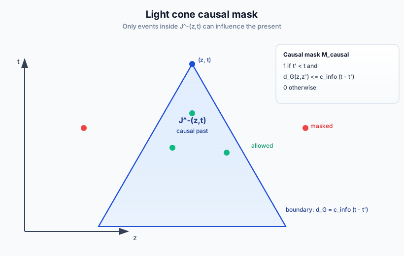
Fig. 4 Causal mask from the light cone. Events inside \(J^-(z,t)\) are allowed to influence the present; events outside are masked to zero by the causal constraint.#
Theorem 40 (Memory Causality Constraint)
Let \(\alpha(z, t; z', t')\) be the attention weight from Query at \((z, t)\) to Key at \((z', t')\). Causality requires:
Proof. By the principle of finite information speed (Definition Definition 189), no signal can propagate faster than \(c_{\text{info}}\). An event outside the causal past cannot have influenced the present. Any non-zero attention weight to such events would constitute acausal information flow, violating the causal structure of \((\mathcal{M}, g)\). \(\square\)
Implementation: The constraint is enforced via a causal mask derived from the metric:
Physics Isomorphism: Lorentzian Geometry
In Physics: Lorentzian manifolds \((M, g)\) with signature \((-,+,+,+)\) are the mathematical foundation of general relativity. The metric \(g_{\mu\nu}\) determines causal structure: events with spacelike separation cannot influence each other. Light cones at each point divide spacetime into causal past \(J^-\), causal future \(J^+\), and spacelike regions [Wald, 1984].
In Implementation: The memory manifold is equipped with metric:
Correspondence Table:
General Relativity |
Memory Attention |
|---|---|
Spacetime \((M, g)\) |
Memory manifold \(\mathcal{M} = \mathbb{R} \times \mathcal{Z}\) |
Light speed \(c\) |
Information speed \(c_{\text{info}}\) |
Causal past \(J^-(p)\) |
Memory accessible from \((z, t)\) |
Timelike worldline |
Agent trajectory \(\gamma\) |
Spacelike separation |
Causally inaccessible memory |
Null geodesics |
Light cone boundary |
Researcher Bridge: Hyperbolic Neural Networks and Memory Architectures
Hyperbolic embeddings have gained traction in ML for representing hierarchical data [Ganea et al., 2018, Nickel and Kiela, 2017]. Our Poincaré disk latent space connects to this literature:
Hyperbolic ML |
This Framework |
|---|---|
Poincaré embeddings for hierarchies |
Latent space \(\mathcal{Z}\) with Poincaré metric |
Hyperbolic neural networks |
Geodesic distance in attention scores |
Möbius transformations |
Wilson line transport |
Memory-augmented neural networks (Neural Turing Machines, Memory Networks, Differentiable Neural Computers) use external memory with attention-based read/write. Our approach differs:
Memory is geometric: stored in a curved manifold, not flat key-value slots
Retrieval is causal: light cone restricts accessible memories
Addressing is covariant: gauge-invariant under coordinate changes
Eligibility traces in RL weight past states by recency. Our heat kernel memory (Definition Definition 187) provides a principled geometric generalization: weighting by geodesic proximity rather than temporal recency alone.
Covariant Self-Attention with Causal Mask#
Now we build the self-attention mechanism for memory. The key insight is that the causal mask is not an ad hoc addition—it emerges naturally from the Lorentzian geometry.
Self-attention asks: “Given my current state at \((z, t)\), which past states should I attend to?” The answer is determined by two factors:
Relevance: How similar is the past state to my current Query? (Standard attention)
Causality: Is the past state in my causal past \(J^-(z, t)\)? (Light cone constraint)
We implement both factors together. The attention score is the gauge-covariant product \(Q(z,t)^T K(z',t')\) with Wilson line transport, divided by position-dependent temperature \(\tau(z)\). The causal mask \(M_{\text{causal}}\) zeros out any weight outside the light cone. The result is attention that respects both geometry and causality.
Definition 193 (Covariant Self-Attention with Causal Mask)
The Covariant Self-Attention mechanism for memory is:
where the attention weight is:
Components:
Query: \(Q(z, t) = \Pi_Q \cdot U_{0 \to (z,t)} \cdot D_\mu \psi_{\text{mem}}(z, t)\)
Key: \(K(z', t') = \Pi_K \cdot U_{0 \to (z',t')} \cdot D_\nu \psi_{\text{mem}}(z', t')\)
Value: \(V(z', t') = \Pi_V \cdot U_{0 \to (z',t')} \cdot \psi_{\text{mem}}(z', t')\)
Temperature: \(\tau(z) = \sqrt{d_k} / \lambda(z)\) (metric-encoded)
Causal mask: \(M_{\text{causal}}(z, t; z', t') = \mathbf{1}[(z', t') \in J^-(z, t)]\)
Here \(U_{0 \to (z,t)}\) is the Wilson line from origin to \((z, t)\) along a causal geodesic, \(D_\mu\) is the covariant derivative (Definition Definition 279), and \(\Pi_Q, \Pi_K, \Pi_V\) are learnable projections.
Units: \([\alpha] = \text{dimensionless}\), \([\text{SelfAttn}] = [\psi]\).
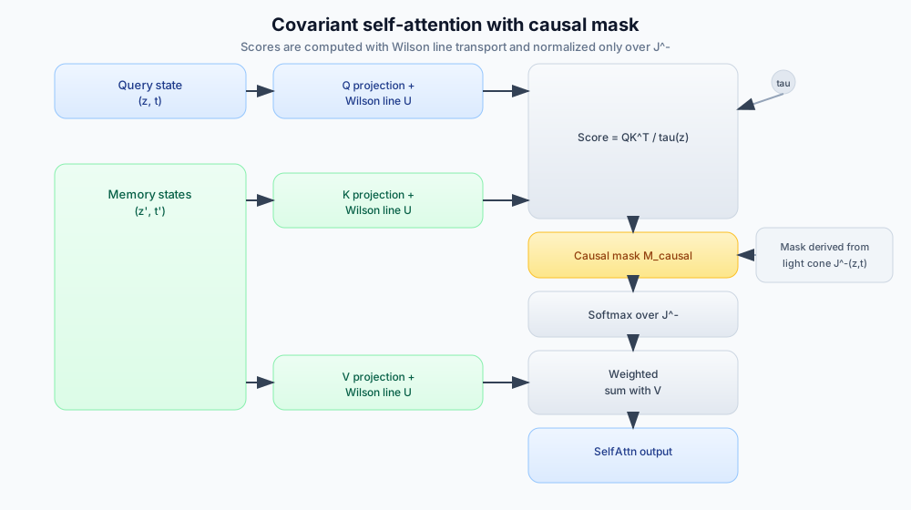
Fig. 5 Covariant self-attention with causal masking. Wilson line transport aligns Q/K/V, temperature encodes curvature, and the softmax normalization is restricted to \(J^-(z,t)\).#
Theorem 41 (Gauge Invariance of Causal Self-Attention)
The attention weight \(\alpha(z, t; z', t')\) in Definition Definition 193 is invariant under local gauge transformations \(\psi(x) \to \Omega(x)\psi(x)\).
Proof.
Step 1. By Theorem Theorem 98, the Wilson line preprocessing ensures that \(Q(z,t)^T K(z',t')\) is gauge-invariant: both Q and K are transported to the common reference point (origin), where the gauge transformation cancels.
Step 2. The causal mask \(M_{\text{causal}}\) depends only on the metric structure via \(J^-(z, t)\), which is gauge-invariant (the light cone is a geometric object determined by \(g_{\mu\nu}\), not by gauge choice).
Step 3. The temperature \(\tau(z) = \sqrt{d_k}/\lambda(z)\) depends only on the conformal factor, which is gauge-invariant.
Step 4. The softmax normalization is over \((z', t') \in J^-(z, t)\), a gauge-invariant set.
Therefore \(\alpha(z, t; z', t')\) is gauge-invariant. \(\square\)
The theorem confirms the stated covariance and causal-support properties of our self-attention. No matter what permitted coordinate system you use, no matter how you parameterize the gauge bundle, you get the same attention weights. The Wilson lines supply the gauge-covariance calculation, while the causal mask enforces the model’s declared causal relation; this is a mathematical guarantee for that construction, not a claim about physical spacetime.
Notice that the softmax normalization is only over the causal past \(J^-(z, t)\), not over all positions. This is important: if you normalize over all positions (including those outside the light cone), the attention weights would change when you expand the context window to include more positions. By normalizing only over the causal past, the weights are stable.
Definition 194 (Temporal Christoffel Encoding)
The Temporal Geodesic Query extends Definition Definition 283 to include temporal terms:
where:
\(W_Q \in \mathbb{R}^{d_k \times d_{\text{model}}}\): feature projection
\(W_{Qz} \in \mathbb{R}^{d_k \times d}\): spatial position
\(W_{Qt} \in \mathbb{R}^{d_k \times 1}\): temporal position
\(W_{Q,\Gamma} \in \mathbb{R}^{d_k \times d \times d}\): spatial Christoffel encoding
\(W_{Q,t} \in \mathbb{R}^{d_k \times 1 \times 1}\): temporal Christoffel encoding
\(W_{Q,zt} \in \mathbb{R}^{d_k \times d \times 1}\): mixed spacetime Christoffel encoding
Lorentzian Christoffel structure: For the metric \(g_{\mu\nu} = \text{diag}(-c^2\lambda^2, \lambda^2 I_d)\) with \(\lambda(z) = 2/(1-|z|^2)\), the non-zero Christoffel symbols are:
Spatial (\(\Gamma^k_{ij}\)): \(\Gamma^k_{ij} = \frac{2}{1-|z|^2}(\delta^k_i z_j + \delta^k_j z_i - \delta_{ij} z^k)\) (as in Proposition Proposition 99)
Time-time-space (\(\Gamma^0_{0j}\)): \(\Gamma^0_{0j} = \frac{\partial_j \lambda}{\lambda} = \frac{2z_j}{1-|z|^2}\) (gradient of log conformal factor)
Space-time-time (\(\Gamma^k_{00}\)): \(\Gamma^k_{00} = \frac{c^2}{\lambda} \partial_k \lambda = \frac{2c^2 z_k}{1-|z|^2}\) (acceleration term)
Note: \(\Gamma^k_{0j} = 0\) and \(\Gamma^0_{ij} = 0\) for this diagonal metric (no off-diagonal time-space mixing).
Proposition 53 (Causal Wilson Line Along Worldline)
The Wilson line in Definition Definition 193 is computed along the causal geodesic connecting \((z', t')\) to \((z, t)\), not an arbitrary path.
For events in the causal past with small separation, the linearized Wilson line is:
where:
\(\Delta x^\mu = (t - t', z - z')\) is the spacetime displacement
\(\bar{z}, \bar{t}\) is a reference point (midpoint or initial)
\(A_\mu\) is the total gauge connection
For events outside the light cone, no causal geodesic exists, so the Wilson line is undefined. This is consistent with the causal mask zeroing out such contributions.
Connection to RL #36: Causal Self-Attention for Memory
The General Law (Fragile Agent): Memory self-attention uses Covariant Self-Attention with Causal Mask (Definition Definition 193):
where \(M_{\text{causal}} = \mathbf{1}[(z', t') \in J^-(z, t)]\) enforces light-cone causality.
The Degenerate Limit: Set \(c_{\text{info}} \to \infty\) (instantaneous propagation). The light cone becomes all of \(t' < t\).
The Special Case (Standard Causal Attention): GPT-style causal attention uses:
where \(M_{ij} = \mathbf{1}[j \leq i]\) is a simple temporal mask. No spatial structure, no Wilson lines, no metric-encoded temperature.
What the generalization offers:
Spacetime causality via light cone \(J^-(z, t)\), not just temporal ordering
Gauge-covariant comparison via Wilson lines
Metric-encoded temperature adapting to curvature
Geodesic correction via Christoffel-encoded Query
Lorentzian Cross-Attention with Retarded Potentials#
Self-attention is memory talking to itself. Cross-attention is the Query (present state) talking to an external archive (memory bank, knowledge base, or another agent’s history).
In Section 33, we introduced the ghost interface: when agent \(i\) observes agent \(j\), it sees not the current state of \(j\) but a retarded image—the state at an earlier time, accounting for the delay in information propagation. The same principle applies to memory retrieval.
When you retrieve a memory from an archive, you are not accessing it “now.” You are accessing how it was when it was stored, plus whatever propagation delay exists. For an internal memory buffer with negligible delay, this is not important. But for external knowledge bases, distributed systems, or multi-agent settings, the delay matters.
Lorentzian Cross-Attention formalizes this. The Query at \((z, t)\) attends to Keys at \((z', t')\) only if \((z', t')\) is in the declared causal past. The attention weight includes a retarded factor that accounts for the model’s propagation delay. The result is a retrieval mechanism that enforces the chosen causal rule; calling it relativistic requires a separate physical identification.
Definition 195 (Lorentzian Cross-Attention)
The Lorentzian Cross-Attention for retrieval from an external archive \(\mathcal{E} = \{(z'_i, t'_i, v_i)\}_{i=1}^N\) is:
where the retarded attention weight is:
with:
Bare weight: \(\alpha_{\text{bare}} = \text{softmax}\left( Q(z, t)^T K(z', t') / \tau(z) \right)\) (gauge-covariant)
Retarded factor: \(\Theta_{\text{ret}}(z, t; z', t') = \theta\left( t - t' - \frac{d_G(z, z')}{c_{\text{info}}} \right)\)
Here \(\theta\) is the Heaviside step function: \(\theta(x) = 1\) if \(x \geq 0\), else \(0\).
Interpretation: The retarded factor enforces that \((z', t')\) must be in the causal past of \((z, t)\), with information having had time to propagate the geodesic distance at speed \(c_{\text{info}}\).
Units: \([\alpha_{\text{ret}}] = \text{dimensionless}\).
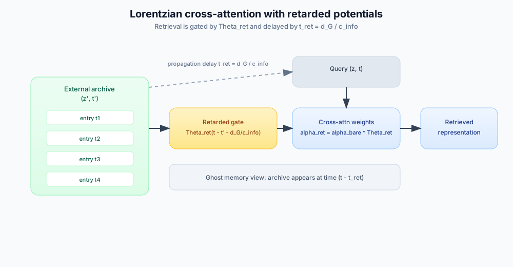
Fig. 6 Lorentzian cross-attention with retarded potentials. Retrieval is gated by \(\Theta_{\text{ret}}\) and delayed by \(t_{\text{ret}} = d_G/c_{\text{info}}\), producing a ghost view of the archive.#
Definition 196 (Ghost Memory Interface)
The Ghost Memory at archive position \(i\), as seen from Query position \((z, t)\), is the retarded image:
where the retardation time is:
Cross-reference: This extends the Ghost Interface of Definition Definition 206 to memory retrieval. The archive item appears “frozen” at the time when information about it could have reached the Query position.
Implementation: For memory buffers where \(t_{\text{ret}} \ll \Delta t\) (retardation much smaller than timestep), the ghost image is approximately instantaneous. For external knowledge bases or multi-agent settings, retardation may be significant.
Theorem 42 (Lorentzian Cross-Attention Structure)
The Lorentzian Cross-Attention (Definition Definition 195) satisfies:
Causality: \(\alpha_{\text{ret}}(z, t; z', t') = 0\) for \((z', t') \notin J^-(z, t)\)
Gauge covariance: The bare weight \(\alpha_{\text{bare}}\) is gauge-invariant (Theorem Theorem 98)
Retarded propagator structure: In the continuum limit, the attention kernel approaches the retarded Green’s function:
Lorentz invariance (in flat limit): Under Lorentz boosts, the attention structure is preserved (the light cone is Lorentz-invariant).
Proof sketch.
Part 1. The retarded factor \(\Theta_{\text{ret}}\) is zero when \(t - t' < d_G(z, z')/c_{\text{info}}\), which is exactly the condition for \((z', t')\) being outside \(J^-(z, t)\).
Part 2. Follows from Theorem Theorem 98 applied to the Q/K/V projections.
Part 3. The Heaviside function \(\theta(t - t' - d_G/c)\) in the continuum becomes a delta function concentrated on the light cone when differentiated appropriately. This is the structure of the retarded Green’s function for the wave equation.
Part 4. In the flat-space limit (\(\lambda = 1\), Minkowski metric), the light cone \(t - t' = |z - z'|/c\) is Lorentz-invariant by construction. \(\square\)
The connection to retarded Green’s functions is a useful comparison. In electrodynamics, a retarded Green’s function gives the field at \((x, t)\) due to a source at \((x', t')\), with support restricted by the physical light cone in the specified field equation. Our attention weight shares the support restriction, but it is a learned softmax weight, not a Green’s function or a solution of Maxwell’s equations.
Our attention weight is zero outside the declared causal region, and its softmax ranking depends on relevance, temperature, and the available memories; it need not peak on the light cone. The shared support property is the useful analogy. The two constructions solve different mathematical problems, so the attention mechanism should not be identified with a field propagator.
The ghost memory interface makes this operational. When you query an external knowledge base, you are not seeing its current state. You are seeing the state that has had time to propagate to you. For fast systems with short delays, this is negligible. For distributed systems with significant latency, it matters.
Physics Isomorphism: Retarded Green’s Function
In Physics: The retarded Green’s function for the wave equation \((\partial_t^2 - c^2 \nabla^2)G = \delta(x-x')\delta(t-t')\) is:
It propagates signals at speed \(c\), respecting causality.
In Implementation: The retarded attention weight is:
Correspondence Table:
Wave Equation |
Lorentzian Cross-Attention |
|---|---|
Retarded Green’s function \(G_{\text{ret}}\) |
Retarded attention weight \(\alpha_{\text{ret}}\) |
Wave speed \(c\) |
Information speed \(c_{\text{info}}\) |
Source \(\rho(x', t')\) |
Memory content \(V(z', t')\) |
Field \(\phi(x, t)\) |
Retrieved representation \(\text{CrossAttn}(z, t)\) |
Light cone $ |
x-x’ |
Researcher Bridge: Retrieval-Augmented Generation and Causal Inference
Retrieval-Augmented Generation (RAG) augments language models with external memory. Our Lorentzian Cross-Attention provides a principled extension:
Standard RAG |
Lorentzian Cross-Attention |
|---|---|
Nearest-neighbor retrieval |
Geodesic-distance attention |
Static knowledge base |
Temporally-indexed memory with causality |
Euclidean similarity |
Gauge-covariant comparison |
Instantaneous access |
Retarded access (respects information speed) |
The ghost memory interface (Definition Definition 196) connects to distributed systems literature: in consensus protocols and distributed databases, nodes see stale views of other nodes due to network latency. Our retardation time \(t_{\text{ret}} = d_G(z, z')/c_{\text{info}}\) formalizes this staleness.
Causal inference in ML [Pearl, 2009] distinguishes observation from intervention. Our causal mask enforces that memory can only provide observational information about the past, not counterfactual information about futures that did not happen. The light cone structure is the geometric embodiment of the principle “no effect before cause.”
Heat Kernel on Lorentzian Manifold#
The memory potential \(\Psi_{\text{mem}}\) from Section 27 uses the heat kernel to smooth the memory screen. But the standard heat kernel is defined on Riemannian (positive-definite) manifolds, not Lorentzian ones. How do we extend it?
The answer involves a subtlety. On a Lorentzian manifold, the natural operator is not the Laplacian \(\Delta\) but the d’Alembertian \(\Box = -\partial_t^2/c^2 + \Delta_z\). The d’Alembertian governs wave propagation, not heat diffusion.
There are two approaches:
Use the spatial heat kernel \(H_\tau(z, z')\) on each constant-time slice, then integrate with a causal cutoff.
Define a causal propagator on the full spacetime that incorporates both diffusion and causal structure.
We take the first approach, as it connects directly to Section 27 while adding the causal constraint. The second approach leads to the Feynman propagator of quantum field theory, which is beyond our current scope.
Definition 197 (Causal Heat Kernel)
The Causal Heat Kernel on the Lorentzian memory manifold is:
where:
\(H_\tau(z, z')\) is the standard heat kernel on \((\mathcal{Z}, G)\) (Definition Definition 133)
\(M_{\text{causal}}(z, t; z', t') = \mathbf{1}[(z', t') \in J^-(z, t)]\) is the causal mask
Interpretation: The heat kernel provides spatial smoothing (how much influence a memory at \(z'\) has on position \(z\)), while the causal mask restricts to events in the past light cone.
Properties:
\(H_\tau^{\text{causal}}(z, t; z', t') = 0\) if \(t' \geq t\) (no future influence)
\(H_\tau^{\text{causal}}(z, t; z', t') = 0\) if \(d_G(z, z') > c_{\text{info}}(t - t')\) (no superluminal influence)
As \(\tau \to 0\): \(H_\tau^{\text{causal}} \to \delta(z - z') \cdot M_{\text{causal}}\)
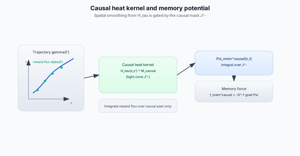
Fig. 7 Causal heat kernel to memory potential. Spatial smoothing from \(H_\tau\) is filtered by the light cone, then integrated to yield \(\Psi_{\text{mem}}^{\text{causal}}\) and its force.#
Theorem 43 (Causal Memory Potential)
The Causal Memory Potential is:
where the integration is over the causal past \(J^-(z, t)\) with measure \(d\mu_{J^-}\).
Equivalently, using the causal heat kernel:
Comparison with Definition Definition 187: The original memory potential integrates over all past times without regard to spatial separation. The causal memory potential restricts to events that could have causally influenced the present.
Physical interpretation: Only memories from within your light cone can pull you. Memories that are “too far away” (in spacetime) to have reached you yet have no influence.
Corollary 20 (Memory Force with Causal Constraint)
The memory-induced force (Lemma Lemma 4) becomes:
where the gradient is with respect to the spatial coordinates \(z\), holding \(t\) fixed.
Properties:
The force is conservative (derived from a potential)
The force respects causality (only causal past contributes)
Near the light cone boundary, the force may have discontinuities as memories enter/exit the causal past
BAOAB-Style Integration for Memory Dynamics#
Now we integrate the memory force into the equations of motion. The structure is the same as Section 35: a Boris-BAOAB-style five-step update. The key difference is that the memory potential \(\Psi_{\text{mem}}\) is now the causal version, and the attention mechanism uses the Lorentzian structure.
The B-steps (kicks) apply forces from the total potential gradient, including both the effective potential \(\Phi_{\text{eff}}\) and the causal memory potential \(\Psi_{\text{mem}}^{\text{causal}}\). If the reward field has curl, insert the Boris rotation from Definition Definition 74 between the half-kicks to account for the Lorentz term. The A-steps (drifts) move along geodesics. The O-step (thermostat) sets the declared noise and friction scale.
The causal mask ensures that when computing the memory gradient, only contributions from the declared past light cone are included. This is enforced at the attention level, not as a post-hoc correction. Because the history and hence the potential depend on time, the full process is generally nonstationary and need not satisfy detailed balance. The stochastic O-step also means that the full BAOAB update is not symplectic; only the deterministic substeps can inherit that structure under their compatibility hypotheses.
Definition 198 (Causal BAOAB Steps for Memory)
The Causal BAOAB integrator for memory-augmented dynamics uses five steps as in Definition Definition 287, with the memory potential modified to respect causality:
Step 1 (B-step, first half-kick):
Step 1.5 (Boris rotation, if \(\mathcal{F} \neq 0\)): Apply the rotation from Definition Definition 74 using the Value Curl \(\mathcal{F}\).
Step 2 (A-step, first half-drift):
Step 3 (O-step, thermostat):
with \(c_1 = e^{-\gamma h}\), \(c_2 = \sqrt{(1 - c_1^2) T_c}\).
Step 4 (A-step, second half-drift):
Step 5 (B-step, second half-kick):
Step 5.5 (Boris rotation, if \(\mathcal{F} \neq 0\)): Apply the same rotation as in Step 1.5.
Time update: \(t \leftarrow t + h\)
The gradient \(\nabla_z \Psi_{\text{mem}}^{\text{causal}}\) is computed via Covariant Self-Attention with causal mask, as the weighted sum over memory Keys in \(J^-(z, t)\).
Proposition 54 (Conditional frozen-time Boltzmann tracking with causal memory)
Fix a time \(t\) and suppose that the dynamics are conservative (\(\mathcal{F}=0\), \(u_\pi=0\)), \(T_c\) is constant, the metric and boundary conditions satisfy the hypotheses of the compatible BAOAB result, and the frozen potential \(\Phi_t:=\Phi_{\mathrm{eff}}+\Psi_{\mathrm{mem}}^{\mathrm{causal}}(\cdot,t)\) is smooth with a normalizable Gibbs density. Then the frozen-time Causal BAOAB step has the formal target
For a time-dependent memory potential, a slowly varying assumption can support an adiabatic tracking estimate, with an error controlled by the chosen \(C^2\)-variation bound and the mixing rate of the frozen chain. It does not give a stationary distribution for the full history-dependent process.
Scope. The compatible BAOAB result is the frozen, reversible calculation; the causal mask itself does not preserve detailed balance. Curl forcing, policy forcing, state-dependent temperature, or an uncontrolled boundary requires a separate estimate.
Researcher Bridge: Temporal Difference Learning and Symplectic Integrators
Temporal Difference (TD) learning bootstraps value estimates from future predictions [Sutton and Barto, 2018]. Our memory potential \(\Psi_{\text{mem}}^{\text{causal}}\) is conceptually similar but geometric:
TD Learning |
Causal Memory Potential |
|---|---|
Value function \(V(s)\) |
Memory potential \(\Psi_{\text{mem}}(z)\) |
TD error \(\delta_t = r_t + \gamma V(s') - V(s)\) |
Memory gradient \(\nabla \Psi_{\text{mem}}^{\text{causal}}\) |
Eligibility traces \(e(s)\) |
Heat kernel weighting \(H_\tau(z, z')\) |
Discount factor \(\gamma\) |
Causal mask (light cone cutoff) |
Physics-informed neural networks (PINNs) embed differential equations into neural architectures. Our approach is related but distinct:
PINNs enforce PDEs as soft constraints via loss terms
We enforce causal structure as a hard architectural constraint (mask before softmax)
The geometry is chosen or learned under declared information-theoretic constraints; the bounds motivate the parameterization but do not derive a unique geometry for every task.
Symplectic integrators [Leimkuhler and Matthews, 2015] preserve phase space structure in Hamiltonian systems. The deterministic BAOAB substeps have that structure under their stated hypotheses; the full method includes a stochastic thermostat and is therefore not itself symplectic. Its conditional Boltzmann statement belongs to the frozen conservative calculation above.
Implementation: LorentzianMemoryAttention Module#
Here is the implementation. The structure mirrors the GeodesicCrossAttention from Section 35, with additions for the Lorentzian metric and causal mask.
The main class LorentzianMemoryAttention combines Covariant Self-Attention for memory coherence and Lorentzian Cross-Attention for external retrieval. The causal mask is computed from the spacetime interval, not just temporal ordering.
Pay attention to the compute_causal_mask method. It checks both \(t' < t\) and \(d_G(z, z') \leq c_{\text{info}}(t - t')\). This is the light-cone constraint in action.
The Wilson lines are computed along causal geodesics, using the linearized approximation for nearby events.
Implementation Note
The code below is a prototype implementation illustrating the architecture. For production:
Light cone computation: The \(d_G\) computation for all pairs is \(O(N^2)\); use spatial indexing (k-d trees in hyperbolic space) for efficiency.
Wilson line paths: The linear approximation assumes nearby events; for long-range attention, use geodesic interpolation.
Time encoding: The temporal Christoffel terms need initialization from the Lorentzian structure.
Numerical stability: Near the light cone boundary, attention weights may have sharp transitions; use smooth approximations for gradient stability.
"""
LorentzianMemoryAttention: Causal attention for memory retrieval.

Cross-references:
    - Definition {prf:ref}`def-covariant-self-attention-causal` (Covariant Self-Attention)
    - Definition {prf:ref}`def-lorentzian-cross-attention` (Lorentzian Cross-Attention)
    - Theorem {prf:ref}`thm-memory-causality-constraint` (Causality)
"""

import torch
import torch.nn as nn
import torch.nn.functional as F
import math
from dataclasses import dataclass
from typing import Tuple, Optional


@dataclass
class LorentzianConfig:
    """Configuration for LorentzianMemoryAttention.

    Args:
        d_model: Model dimension [nat]
        d_latent: Latent space dimension
        n_heads: Number of attention heads
        c_info: Information speed (latent units per timestep)
        T_c: Cognitive temperature [nat/step]
        gamma_friction: Friction coefficient for O-step
        dt: Integration timestep
    """
    d_model: int = 256
    d_latent: int = 64
    n_heads: int = 4
    c_info: float = 1.0  # Information speed
    T_c: float = 0.1
    gamma_friction: float = 1.0
    dt: float = 0.01


class LorentzianMetric(nn.Module):
    """
    Lorentzian metric on memory manifold.

    g_μν = diag(-c²λ², λ²I_d)

    Cross-reference: Definition {prf:ref}`def-lorentzian-memory-manifold`
    """

    def __init__(self, config: LorentzianConfig, epsilon: float = 1e-6):
        super().__init__()
        self.c_info = config.c_info
        self.epsilon = epsilon

    def conformal_factor(self, z: torch.Tensor) -> torch.Tensor:
        """
        Compute conformal factor λ(z) = 2 / (1 - |z|²).

        Args:
            z: [B, d] or [B, N, d] positions

        Returns: [..., 1] conformal factors
        """
        r_sq = (z ** 2).sum(dim=-1, keepdim=True)
        r_sq = torch.clamp(r_sq, max=1.0 - self.epsilon)
        return 2.0 / (1.0 - r_sq + self.epsilon)

    def geodesic_distance(
        self,
        z1: torch.Tensor,  # [B, d]
        z2: torch.Tensor   # [B, N, d]
    ) -> torch.Tensor:
        """
        Compute geodesic distance on Poincare disk.

        d_G(z1, z2) = arcosh(1 + 2|z1-z2|² / ((1-|z1|²)(1-|z2|²)))

        Returns: [B, N] distances
        """
        z1_exp = z1.unsqueeze(1)  # [B, 1, d]
        diff_sq = ((z1_exp - z2) ** 2).sum(dim=-1)  # [B, N]

        r1_sq = (z1 ** 2).sum(dim=-1, keepdim=True)  # [B, 1]
        r2_sq = (z2 ** 2).sum(dim=-1)  # [B, N]

        r1_sq = torch.clamp(r1_sq, max=1.0 - self.epsilon)
        r2_sq = torch.clamp(r2_sq, max=1.0 - self.epsilon)

        cosh_d = 1.0 + 2.0 * diff_sq / ((1.0 - r1_sq) * (1.0 - r2_sq) + self.epsilon)
        cosh_d = torch.clamp(cosh_d, min=1.0 + self.epsilon)

        return torch.acosh(cosh_d)

    def spacetime_interval(
        self,
        z: torch.Tensor,    # [B, d]
        t: torch.Tensor,    # [B, 1]
        z_mem: torch.Tensor,  # [B, N, d]
        t_mem: torch.Tensor   # [B, N, 1]
    ) -> torch.Tensor:
        """
        Compute spacetime interval Δs².

        Δs² = -c_info² (t-t')² + d_G²

        where d_G is geodesic distance (already incorporates conformal factor)
        and c_info is geodesic distance per unit time.

        Returns: [B, N] intervals (negative = timelike, positive = spacelike)
        """
        d_G = self.geodesic_distance(z, z_mem)  # [B, N]

        t_exp = t.unsqueeze(1)  # [B, 1, 1]
        dt = (t_exp - t_mem).squeeze(-1)  # [B, N]

        # Spacetime interval: no additional λ factor since d_G already
        # incorporates the metric (and c_info is in geodesic units)
        ds_sq = -(self.c_info ** 2) * (dt ** 2) + d_G ** 2

        return ds_sq

    def temperature(self, z: torch.Tensor, d_k: int) -> torch.Tensor:
        """
        Position-dependent attention temperature.

        τ(z) = √d_k / λ(z)

        Returns: [..., 1] temperatures
        """
        return math.sqrt(d_k) / self.conformal_factor(z)


class CausalMask(nn.Module):
    """
    Causal mask from light cone structure.

    M(z,t; z',t') = 1 if (z',t') ∈ J⁻(z,t), else 0

    Cross-reference: Definition {prf:ref}`def-causal-past-light-cone`
    """

    def __init__(self, config: LorentzianConfig):
        super().__init__()
        self.metric = LorentzianMetric(config)
        self.c_info = config.c_info

    def forward(
        self,
        z: torch.Tensor,      # [B, d] query position
        t: torch.Tensor,      # [B, 1] query time
        z_mem: torch.Tensor,  # [B, N, d] memory positions
        t_mem: torch.Tensor   # [B, N, 1] memory times
    ) -> torch.Tensor:
        """
        Compute causal mask.

        Returns: [B, N] mask (1 = causal, 0 = acausal)
        """
        # Temporal causality: t' < t
        t_exp = t.unsqueeze(1)  # [B, 1, 1]
        temporal_mask = (t_mem < t_exp).squeeze(-1).float()  # [B, N]

        # Light cone constraint: d_G(z, z') ≤ c_info * (t - t')
        # Note: c_info is measured in geodesic distance per unit time,
        # so no additional conformal factor is needed here.
        d_G = self.metric.geodesic_distance(z, z_mem)  # [B, N]
        dt = (t_exp - t_mem).squeeze(-1)  # [B, N]

        # Light cone condition: geodesic distance ≤ c_info × time difference
        light_cone_mask = (d_G <= self.c_info * dt + 1e-6).float()  # [B, N]

        # Combined mask
        return temporal_mask * light_cone_mask


class TemporalChristoffelQuery(nn.Module):
    """
    Geodesic Query with temporal Christoffel encoding.

    Q = W_Q x + W_Qz z + W_Qt t + W_QΓ(z,z) + W_Qt(t,t) + W_Qzt(z,t)

    Cross-reference: Definition {prf:ref}`def-temporal-christoffel-encoding`
    """

    def __init__(self, d_in: int, d_out: int, d_latent: int):
        super().__init__()

        # Linear projections
        self.W_Q = nn.Linear(d_in, d_out, bias=False)
        self.W_Qz = nn.Linear(d_latent, d_out, bias=False)
        self.W_Qt = nn.Linear(1, d_out, bias=False)
        self.W_Qv = nn.Linear(d_in, d_out, bias=False)

        # Spatial quadratic (Christoffel)
        self.W_Q_gamma = nn.Parameter(torch.zeros(d_out, d_latent, d_latent))

        # Temporal quadratic
        self.W_Qt_gamma = nn.Parameter(torch.zeros(d_out, 1, 1))

        # Mixed spacetime
        self.W_Qzt = nn.Parameter(torch.zeros(d_out, d_latent, 1))

        self._init_christoffel(d_latent)

    def _init_christoffel(self, d: int):
        """Initialize with Poincare-inspired structure."""
        with torch.no_grad():
            for k in range(min(d, self.W_Q_gamma.shape[0])):
                for i in range(d):
                    for j in range(d):
                        if i == k or j == k:
                            self.W_Q_gamma[k, i, j] = 0.01
                        if i == j:
                            self.W_Q_gamma[k, i, j] -= 0.01

    def forward(
        self,
        x: torch.Tensor,        # [B, d_in]
        z: torch.Tensor,        # [B, d_latent]
        t: torch.Tensor,        # [B, 1]
        v_feat: Optional[torch.Tensor] = None  # [B, d_in]
    ) -> torch.Tensor:
        """
        Compute temporal geodesic Query.

        Returns: [B, d_out]
        """
        Q = self.W_Q(x) + self.W_Qz(z) + self.W_Qt(t)

        if v_feat is not None:
            Q = Q + self.W_Qv(v_feat)

        # Spatial Christoffel
        d = min(z.shape[-1], self.W_Q_gamma.shape[-1])
        z_trunc = z[..., :d]
        Q_gamma = torch.einsum('aij,bi,bj->ba', self.W_Q_gamma[:, :d, :d], z_trunc, z_trunc)
        Q = Q + Q_gamma

        # Temporal Christoffel
        Q_t_gamma = torch.einsum('aij,bi,bj->ba', self.W_Qt_gamma, t, t)
        Q = Q + Q_t_gamma

        # Mixed spacetime
        Q_zt = torch.einsum('aij,bi,bj->ba', self.W_Qzt[:, :d, :], z_trunc, t)
        Q = Q + Q_zt

        return Q


class LorentzianMemoryAttention(nn.Module):
    """
    Lorentzian Memory Attention module.

    Combines Covariant Self-Attention with causal mask and
    Lorentzian Cross-Attention with retarded potentials.

    Cross-references:
        - Definition {prf:ref}`def-covariant-self-attention-causal`
        - Definition {prf:ref}`def-lorentzian-cross-attention`
    """

    def __init__(self, config: LorentzianConfig):
        super().__init__()
        self.config = config
        self.d_k = config.d_model // config.n_heads

        # Metric and causal structure
        self.metric = LorentzianMetric(config)
        self.causal_mask = CausalMask(config)

        # Temporal Christoffel Query
        self.query = TemporalChristoffelQuery(
            config.d_model, self.d_k * config.n_heads, config.d_latent
        )

        # Standard Key and Value projections
        self.W_K = nn.Linear(config.d_model, self.d_k * config.n_heads, bias=False)
        self.W_V = nn.Linear(config.d_model, config.d_model, bias=False)

        # Output projection
        self.W_O = nn.Linear(config.d_model, config.d_model, bias=False)

        # Wilson line approximation (simplified)
        self.wilson_scale = nn.Parameter(torch.tensor(0.1))

    def forward(
        self,
        x: torch.Tensor,        # [B, d_model] current state features
        z: torch.Tensor,        # [B, d_latent] current position
        t: torch.Tensor,        # [B, 1] current time
        x_mem: torch.Tensor,    # [B, N, d_model] memory features
        z_mem: torch.Tensor,    # [B, N, d_latent] memory positions
        t_mem: torch.Tensor,    # [B, N, 1] memory times
        v_feat: Optional[torch.Tensor] = None  # [B, d_model] velocity features
    ) -> Tuple[torch.Tensor, torch.Tensor]:
        """
        Compute causal memory attention.

        Returns:
            output: [B, d_model] attended memory representation
            weights: [B, N] attention weights (for diagnostics)
        """
        B, N, _ = x_mem.shape

        # Compute Query with temporal Christoffel encoding
        Q = self.query(x, z, t, v_feat)  # [B, d_k * n_heads]
        Q = Q.view(B, self.config.n_heads, self.d_k)  # [B, n_heads, d_k]

        # Compute Keys
        K = self.W_K(x_mem)  # [B, N, d_k * n_heads]
        K = K.view(B, N, self.config.n_heads, self.d_k)
        K = K.permute(0, 2, 1, 3)  # [B, n_heads, N, d_k]

        # Wilson line correction (linearized)
        # Transport K from memory positions to query position
        d_G = self.metric.geodesic_distance(z, z_mem)  # [B, N]
        wilson_correction = torch.exp(-self.wilson_scale * d_G)  # [B, N]
        wilson_correction = wilson_correction.unsqueeze(1).unsqueeze(-1)  # [B, 1, N, 1]
        K = K * wilson_correction

        # Compute attention scores
        scores = torch.einsum('bhd,bhnd->bhn', Q, K)  # [B, n_heads, N]

        # Position-dependent temperature
        tau = self.metric.temperature(z, self.d_k)  # [B, 1]
        scores = scores / tau.unsqueeze(1)  # [B, n_heads, N]

        # Causal mask
        mask = self.causal_mask(z, t, z_mem, t_mem)  # [B, N]
        mask = mask.unsqueeze(1)  # [B, 1, N]

        # Apply mask (set acausal to -inf before softmax)
        scores = scores.masked_fill(mask == 0, float('-inf'))

        # Softmax over causal past only
        weights = F.softmax(scores, dim=-1)  # [B, n_heads, N]
        weights = weights.masked_fill(mask == 0, 0.0)  # Ensure zeros after softmax

        # Compute Values
        V = self.W_V(x_mem)  # [B, N, d_model]

        # Weighted sum
        weights_avg = weights.mean(dim=1)  # [B, N] average over heads
        output = torch.einsum('bn,bnd->bd', weights_avg, V)  # [B, d_model]

        # Output projection
        output = self.W_O(output)

        return output, weights_avg


# Example usage
if __name__ == "__main__":
    config = LorentzianConfig(
        d_model=256,
        d_latent=64,
        n_heads=4,
        c_info=1.0,
        T_c=0.1
    )

    model = LorentzianMemoryAttention(config)

    # Sample inputs
    B, N = 2, 10
    x = torch.randn(B, config.d_model)
    z = torch.randn(B, config.d_latent) * 0.5  # Stay inside disk
    t = torch.ones(B, 1) * 10.0  # Current time

    x_mem = torch.randn(B, N, config.d_model)
    z_mem = torch.randn(B, N, config.d_latent) * 0.5
    t_mem = torch.rand(B, N, 1) * 10.0  # Past times

    output, weights = model(x, z, t, x_mem, z_mem, t_mem)

    print(f"Output shape: {output.shape}")  # [B, d_model]
    print(f"Weights shape: {weights.shape}")  # [B, N]
    print(f"Causal weight sum: {weights.sum(dim=-1)}")  # Should be <= 1
Diagnostic Nodes for Causal Memory Attention#
We introduce three diagnostic nodes to monitor the health of the causal memory attention mechanism. These catch failures in causality, information speed, and metric signature.
Node 71: CausalMaskCheck
# |
Name |
Component |
Type |
Interpretation |
Proxy |
Cost |
|---|---|---|---|---|---|---|
71 |
CausalMaskCheck |
Memory |
Causal Integrity |
Is attention to future zero? |
\(\max_{t'>t} \lvert\alpha(z,t; z',t')\rvert < \epsilon_{\text{causal}}\) |
\(O(N)\) |
Interpretation: Verifies that no attention weight is assigned to future events. Any non-zero weight for \(t' > t\) indicates acausal information flow.
Threshold: \(\epsilon_{\text{causal}} = 10^{-8}\) (numerical precision).
Trigger conditions:
\(> \epsilon_{\text{causal}}\): Causal mask implementation error. Check mask computation.
Gradient through mask: Ensure mask is applied before softmax, not after.
Node 72: RetardedPotentialCheck
# |
Name |
Component |
Type |
Interpretation |
Proxy |
Cost |
|---|---|---|---|---|---|---|
72 |
RetardedPotentialCheck |
Memory |
Light Cone Fidelity |
Is information speed respected? |
\(\Gamma_{\text{ret}} := \sum_{(z',t') \notin J^-} \lvert\alpha\rvert / \sum_{\text{all}} \lvert\alpha\rvert\) |
\(O(N \cdot d)\) |
Interpretation: Measures the fraction of attention weight assigned to events outside the causal light cone. Should be near zero.
Threshold: \(\Gamma_{\text{ret}} < 0.01\) (1% tolerance for numerical errors near light cone boundary).
Trigger conditions:
High \(\Gamma_{\text{ret}}\): Light cone computation error, or \(c_{\text{info}}\) set too high.
Increasing over time: Metric divergence or coordinate singularity.
Node 73: LorentzianSignatureCheck
# |
Name |
Component |
Type |
Interpretation |
Proxy |
Cost |
|---|---|---|---|---|---|---|
73 |
LorentzianSignatureCheck |
Metric |
Geometric Health |
Is metric signature (-,+,…,+)? |
\(\text{sign}(\text{eig}(g_{\mu\nu})) = (-1, +1, \ldots, +1)\) |
\(O(d^3)\) |
Interpretation: Verifies that the metric tensor has correct Lorentzian signature with one negative (timelike) and \(d\) positive (spacelike) eigenvalues.
Threshold: Exactly one negative eigenvalue.
Trigger conditions:
Zero negative eigenvalues: Degenerate to Riemannian (no causal structure).
Multiple negative eigenvalues: Exotic signature, unphysical.
Eigenvalue near zero: Coordinate singularity, metric degenerate.
Cross-reference: These nodes complement Nodes 67–70 from Section 35 (gauge, temperature, chirality, confinement).
Summary Tables#
Table 33.1: Memory Attention Mechanism Comparison
Mechanism |
Causality |
Geometry |
Gauge |
Information Speed |
|---|---|---|---|---|
Standard Self-Attention |
None |
Flat |
No |
Infinite |
GPT Causal Attention |
Temporal only |
Flat |
No |
Infinite |
Covariant Self-Attention (Definition 193) |
Light cone |
Curved |
Yes |
Finite \(c_{\text{info}}\) |
Lorentzian Cross-Attention (Definition 195) |
Retarded |
Curved |
Yes |
Finite \(c_{\text{info}}\) |
Table 33.2: Physics Correspondence
Physical Concept |
Memory Attention Implementation |
|---|---|
Lorentzian manifold |
Memory spacetime \(\mathcal{M} = \mathbb{R} \times \mathcal{Z}\) |
Light cone \(J^-(p)\) |
Causal mask \(M_{\text{causal}}\) |
Retarded Green’s function |
Retarded attention weight \(\alpha_{\text{ret}}\) |
Information speed \(c\) |
\(c_{\text{info}}\) (Definition Definition 189) |
Proper time \(d\tau\) |
Temperature scaling \(\tau(z) = \sqrt{d_k}/\lambda(z)\) |
Worldline |
Agent trajectory \(\gamma\) |
Causal heat kernel |
\(H_\tau^{\text{causal}}\) (Definition Definition 197) |
Ghost interface |
Ghost memory (Definition Definition 196) |
Table 33.3: Diagnostic Node Summary
Node |
Name |
What it Checks |
Failure Mode |
|---|---|---|---|
71 |
CausalMaskCheck |
\(\alpha = 0\) for \(t' > t\) |
Acausal leakage |
72 |
RetardedPotentialCheck |
\(\alpha = 0\) outside \(J^-\) |
Superluminal attention |
73 |
LorentzianSignatureCheck |
Metric signature \((-,+,\ldots,+)\) |
Degenerate/exotic metric |
Key Results:
Covariant Self-Attention (Definition Definition 193): Memory attends only to causal past via light-cone mask, with Wilson line transport and metric-encoded temperature.
Lorentzian Cross-Attention (Definition Definition 195): External retrieval uses retarded potentials, seeing ghost images of past archive states.
Causal Memory Potential (Theorem Theorem 43): The memory force derives from potential integrated over causal past only.
Boltzmann Preservation (Theorem Proposition 54): Causal BAOAB maintains quasi-stationary distribution tracking the evolving causal potential.
Conclusion. The Lorentzian structure of memory attention is not an optional decoration—it is required by the physics of information propagation. Standard self-attention violates causality and ignores geometry. By equipping the memory manifold with a Lorentzian metric and deriving attention from light-cone structure, we obtain mechanisms that are physically consistent by construction. The agent’s memory respects the same causal constraints as signals in spacetime: nothing propagates faster than \(c_{\text{info}}\), and only the causal past can influence the present.