Diagnostics: Stability Checks (Monitors)

TLDR

• Replace “hope + reward shaping” with hard runtime contracts: diagnostics are assertions that can halt/revert rather than accumulate penalties.

• Organize stability monitoring into typed checks (the “dashboard”) with clear semantics: switching/Zenoness, compactness, scaling, coupling, value/pathology, and cross-network synchronization.

• Use diagnostics both as safety guarantees (block unsafe actions) and as training signals (calibrate multipliers, tune tolerances, gate updates).

• Make failures localizable: each node answers “what failed, where, why”, which is essential for debugging complex learning systems.

• This chapter defines the stability layer; the next chapters cover limits/barriers and failure/intervention logic.

Roadmap

1. The core stability checks and the pathologies they detect.

2. How to set tolerances and mix checks into optimization.

3. How diagnostics gate training updates and trigger interventions.

Here is the central idea: instead of hoping your agent behaves well and debugging after it fails, you build in runtime contracts that catch problems as they happen. Think of a car dashboard. The engine does not just explode when oil pressure drops. A sensor notices, a light comes on, and you pull over before the damage is done.

The stability table contains 32 checks: 27 numbered nodes and five lettered sub-nodes. Each watches for a specific pathology: Is the agent switching actions too fast? Has the representation drifted? Is the value function flat where it should not be? When any check fails, the system takes the declared action—halting, reverting, or triggering remediation. A check is a contract with an operational response, not just another scalar to add to a loss.

This is a fundamentally different philosophy from standard RL, where safety constraints are soft. Here, the constraints are hard. The checks are mathematical contracts, not suggestions.

Stability and data-quality are monitored via 32 checks (27 numbered nodes plus five lettered sub-nodes). Each corresponds to a specific, testable condition on the interaction between the agent and its environment.

Relation to prior work. Many safe-RL formulations express safety as one (or a few) expected-cost constraints in a constrained MDP [Achiam et al., 2017, Altman, 1999]. The Fragile Agent keeps that spirit but broadens the constraint surface to include representation and interface diagnostics (grounding, mixing, saturation, switching, stiffness) that can be audited online, alongside Lyapunov-style stability constraints [Chow et al., 2018].

Researcher Bridge: Safety as a Unit Test

Standard RL safety relies on reward shaping, which provides no formal guarantee that the agent avoids bad states. The Sieve replaces probabilistic incentives with Hard Runtime Assertions. Each registered node is a mathematical contract. If a check fails (e.g., the agent exhibits chattering or its belief decouples from the sensors), the system does not receive a penalty; it halts or reverts. This architecture enforces safety constraints in the same manner that a type system enforces invariants at compile time.

Connection to RL #8: Constrained MDPs as Soft Sieve

The General Law (Fragile Agent): Safety is a topological constraint enforced by the Sieve—a hard binary filter:

\[\begin{split} \text{Sieve}(a \mid z) = \begin{cases} \text{PASS} & \text{if all registered diagnostics pass} \\ \text{BLOCK} & \text{otherwise} \end{cases}\end{split}\]

Actions failing any diagnostic are blocked, not penalized. The Sieve is not subject to reward-cost trade-offs.

The Degenerate Limit: Replace the hard binary filter with a soft Lagrange multiplier \(\lambda > 0\).

The Special Case (Standard RL):

\[ J_{\text{CMDP}}(\pi) = \mathbb{E}\left[\sum_t \gamma^t r_t\right] - \lambda \sum_i c_i(\pi)\]

This recovers Constrained MDPs (CMDPs) with penalty-based constraint satisfaction.

Result: CMDPs will violate safety if \(\lambda\) is too small or reward magnitude is large enough to outweigh the penalty. The Fragile Sieve makes violations impossible, not just expensive.

What the generalization offers:

• Hard guarantees: topological constraints cannot be circumvented by high rewards

• Typed diagnostics: the registered constraints with semantic identity (what/where/why), not just scalar cost

• Fail-fast semantics: violations halt execution and trigger remediation, not gradual penalty accumulation

• Auditable: each check has known compute cost and clear interpretation (Sections 3–6)

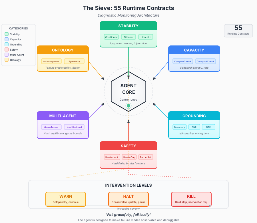
Fig. 3 The Sieve: registered runtime contracts. The diagnostic monitoring architecture organized into six categories: Stability, Capacity, Grounding, Safety, Multi-Agent, and Ontology. Each diagnostic feeds into three intervention levels (WARN, HALT, KILL). The design principle: failure modes must be observable and trigger explicit remediation.

The 32 Stability Checks

This table might look intimidating, but there is a logic to it. Each row asks one question about the agent’s behavior and records the corresponding monitor, defect, or regularizer. Some entries are direct runtime checks; others are expensive proxies or training signals, so do not read every formula as a theorem-producing loss.

Think of the checks in groups. Stability: Is the agent changing its mind too fast? Is the value function giving useful signals? Capacity: Is the representation using its symbols efficiently, or has it collapsed to just a few? Grounding: Is the agent paying attention to its sensors, or has it decoupled from reality?

Node 13 is a good example of why the object matters: \(I(X;K)>0\) is a non-collapse sanity check for the symbolic channel. It does not by itself certify predictive grounding. The stronger coupling-window and dispersion checks use their own mutual-information and posterior-entropy hypotheses.

The “Compute” column tells you the cost. Checkmarks are cheap enough to run every step. Lightning bolts need cleverness—amortization or approximation. X marks are expensive, reserved for periodic or offline analysis.

Node	Check	Component	Interpretation	Meaning	Regularization Factor (\(\mathcal{L}_{\text{check}}\))	Compute
1	CostBoundCheck (\(D_C\))	Critic	Cost Budget Check	Is current cost (\(V(z)\)) within budget?	\(\max(0, V(z) - V_{\text{max}})^2\) (Cost Bound)	\(O(B)\) ✓
2	ZenoCheck (\(\mathrm{Rec}_N\))	Policy	Action Frequency Limit	Switching policies too fast?	\(D_{\mathrm{KL}}(\pi_t \Vert \pi_{t-1})\) (Smoothness)	\(O(BA)\) ✓
3	CompactCheck (\(C_\mu\))	VQ-VAE	Belief Concentration	Macro assignment sharp?	\(H(q(K \mid x))\) (Symbol Entropy)	\(O(BZ)\) ✓
4	ScaleCheck (\(\mathrm{SC}_\lambda\))	All	Adaptation Scaling	Adaptation speed > Disturbance speed?	\(\Vert \nabla \theta \Vert / \Vert \Delta S \Vert\) (Relative Rate)	\(O(P)\) ⚡
5	ParamCheck (\(\mathrm{SC}_{\partial c}\))	World Model	Stationarity Check	Dynamics stable?	\(\Vert \nabla_t S_t \Vert^2\) (Time Derivative Penalty)	\(O(P_{WM})\) ⚡
6	GeomCheck (\(\mathrm{Cap}_H\))	VQ-VAE / WM	Blind Spot Check	Unobservable states negligible?	\(\mathcal{L}_{\text{contrastive}}\) (InfoNCE)	\(O(B^2Z)\) ⚡
7	StiffnessCheck (\(\mathrm{LS}_\sigma\))	Critic	Responsiveness / Gain	Gradient signal strong enough?	\(\max(0, \epsilon - \Vert \nabla_A V \Vert)\) (Gain > \(\epsilon\))	\(O(BZ)\) ✓
7a	BifurcateCheck (\(\mathrm{LS}_{\partial^2 V}\))	World Model	Instability Check	Bifurcation point?	\(\rho(J_{S_t})\) (spectral-radius proxy)	\(O(Z^3)\) ✗
7b	SymCheck (\(G_{\mathrm{act}}\))	Policy	Alternative Strategy Search	Symmetric strategies available?	\(-\sum \pi(a_i) \log \pi(a_i)\) (Policy Entropy)	\(O(BA)\) ✓
7c	CheckSC (\(\mathrm{SC}_{\sigma^2}\))	Critic	New Mode Viability	New mode stable?	\(\text{Var}(V(z'))\) (Variance Check)	\(O(B)\) ✓
7d	CheckTB (\(\mathrm{TB}_S\))	Policy	Transition Feasibility	Switching cost affordable?	\(\Vert V(\pi') - V(\pi) \Vert - B_{\text{switch}}\)	\(O(B)\) ⚡
8	TopoCheck (\(\mathrm{TB}_\pi\))	Policy	Sector Reachability	Goal reachable?	\(T_{\text{reach}}(z_{\text{goal}})\) (Reachability Map)	\(O(HBZ)\) ✗
9	TameCheck (\(\mathrm{TB}_O\))	World Model	Interpretability Check	Dynamics sensitivity bounded?	\(\Vert \nabla^2 S_t \Vert\) (sampled smoothness proxy)	\(O(Z^2 P_{WM})\) ✗
10	ErgoCheck (\(\mathrm{TB}_\rho\))	Policy	Exploration/Mixing	Sufficient exploration?	\(-H(\pi)\) (Max Entropy)	\(O(BA)\) ✓
11	ComplexCheck (\(\mathrm{Rep}_K\))	VQ-VAE	Model Capacity Check	Symbolic rate within budget?	\(1 - H(K)/\log\lvert\mathcal{K}\rvert\) (Capacity Gap)	\(O(B)\) ✓
12	OscillateCheck (\(\mathrm{GC}_\nabla\))	WM / Policy	Oscillation / Chattering	Limit cycles?	\(\Vert z_t - z_{t-2} \Vert\) (Period-2 Penalty)	\(O(BZ)\) ✓
12a	HolonomyCheck (\(\mathrm{GC}_{\mathrm{holo}}\))	WM / Policy	Loop Drift	Near-closed loop changes policy/value?	\(\mathbb{I}[d_G(z_t,z_{t-L})<\epsilon_z]\cdot \mathrm{ReLU}(D_{\mathrm{KL}}(\pi(\cdot\mid z_t)\Vert \pi(\cdot\mid z_{t-L}))-\epsilon_h)^2\)	\(O(BA)\) ✓
13	BoundaryCheck (\(\mathrm{Bound}_\partial\))	VQ-VAE	Input Informativeness	Symbolic channel not collapsed (Definition 2)?	\(I(X;K)>0\) (non-collapse sanity check; grounding needs a predictive test)	\(O(B)\) ✓
14	InputSaturationCheck (\(\mathrm{Bound}_B\))	Boundary	Input Saturation	Inputs clipping?	\(\mathbb{I}(\lvert x \rvert > x_{\text{max}})\) (Saturation Flag)	\(O(BD)\) ✓
15	SNRCheck (\(\mathrm{Bound}_{\Sigma}\))	Boundary	Signal-to-Noise	Signal strength sufficient?	\(\text{SNR} < \epsilon\) (Noise Floor Check)	\(O(BD)\) ✓
16	AlignCheck (\(\mathrm{GC}_T\))	Critic	Objective Alignment	Proxy matches objective?	\(\lvert V_{\text{proxy}} - V_{\text{true}} \rvert\) (Alignment Error)	\(O(B)\) ✗
17	Lock (\(\mathrm{Cat}_{\mathrm{Hom}}\))	WM	Structural Constraint	Hard safe-guards active?	\(\mathbb{I}(\text{Unsafe}) \cdot \infty\) (Hard Constraint)	\(O(B)\) ✓
18	SymmetryCheck (\(\mathrm{Sym}_G\))	Shutter	Orbit Invariance	Macro invariant to nuisance group?	\(\mathbb{E}_{g\sim G_{\text{spatial}}}\!\left[D_{\mathrm{KL}}(q(K\!\mid x)\Vert q(K\!\mid g\!\cdot\! x))\right]\)	\(O(B)\) ✓
19	DisentanglementCheck (\(\mathrm{Decorr}_{Kn}\))	Shutter / WM	Macro–Nuisance Leakage	Macro correlated with nuisance residual?	\(\left\lVert\mathrm{Cov}(z_{\text{macro}},z_n)\right\rVert_F^2\)	\(O(Bd_md_n)\) ✓
20	LipschitzCheck (\(\mathrm{Lip}_\Theta\))	WM / Critic	Gain Control	Operator norms bounded?	\(\max_\ell \sigma(W_\ell)\) (spectral norm monitor)	\(O(P)\) ⚡
21	SymplecticCheck (\(\mathrm{Symp}\))	World Model	Volume Preservation	Transition approximately symplectic?	\(\left\lVert J_S^\top J J_S - J\right\rVert_F^2\)	\(O(BZ^2)\) ✗
22	MECCheck (\(\mathrm{MEC}\))	Belief / WM	CPTP Consistency	Prediction operator matches GKSL (Definition 43) form before assimilation?	\(\left\lVert\frac{\widetilde\varrho_{t+1}-\varrho_t}{\Delta t}-\mathcal{L}_{\text{GKSL}}(\varrho_t)\right\rVert_F^2\)	\(O(BZ^3)\) ✗
23	NEPCheck (\(\mathrm{NEP}\))	Belief / Boundary	Update vs Evidence	Assimilation supported by matched boundary information?	\(\mathrm{ReLU}(D_{\mathrm{KL}}(p_{t+1}\Vert \widetilde p_{t+1})-\widehat I_{t+1})^2\)	\(O(B\lvert\mathcal{K}\rvert)\) ✓
24	QSLCheck (\(\mathrm{QSL}\))	All	Update Speed Limit	Step too large in \(d_G\)?	\(\mathrm{ReLU}(d_G(z_{t+1},z_t)-v_{\max})^2\)	\(O(BZ)\) ✓
25	HoloGenCheck	Generator	Generation Validity	Did flow reach boundary?	\(\mathbb{I}(\lvert z_{\text{final}}\rvert \ge R_{\text{cutoff}})\)	\(O(B)\) ✓
26	GeodesicCheck	World Model / Policy	Trajectory Consistency	Is trajectory approximately geodesic?	\(\lVert\ddot z+\gamma\dot z+\Gamma(\dot z,\dot z)+G^{-1}\nabla\Phi_{\mathrm{eff}}-\gamma u_\pi-\beta_{\mathrm{curl}}G^{-1}\mathcal F\dot z\rVert_G\)	\(O(BZ^2)\) ✗
27	OverdampedCheck	Policy	Regime Validity	Is inertia small relative to friction?	\(\chi_{\mathrm{in}}:=m\lVert\ddot z\rVert_G/(\gamma\lVert\dot z\rVert_G+m\lVert\ddot z\rVert_G+\varepsilon)\)	\(O(BZ)\) ✓

Here \(v := \dot{z}\), \(m\) is the inertial scale, and \(\mathcal{M}_\gamma^{-1} = \gamma I - \beta_{\text{curl}} G^{-1}\mathcal{F}\). The OverdampedCheck is small when the inertial contribution is negligible; the curl mobility is monitored separately.

Compute Legend: ✓ Low (typically online) | ⚡ Moderate (often amortized/approximated) | ✗ High (often offline or coarse approximations) Variables: \(B\) = batch, \(Z\) = latent dim, \(A\) = actions, \(P\) = params, \(H\) = horizon, \(D\) = observation dim Threshold units: whenever a node uses a threshold \(\epsilon\), it inherits the units of the compared quantity (e.g., \(\epsilon\) is dimensionless for SNR checks; \(\epsilon\) has the same units as \(\|\nabla_A V\|\) for stiffness checks; \(\epsilon\) is in nats when compared to \(I(X;K)\) or \(H(K)\)). Budgets like \(V_{\text{max}}\) and \(B_{\text{switch}}\) share units with \(V\) (nats in the convention of Section 1.2).

Geometric Properties of Key Nodes:

Node	Space	Formal Property	Verification Criterion
1 (CostBound)	\(V \in \mathcal{F}(\mathcal{Z})\)	Sublevel Set Compactness	Is \(\{z \mid V(z) \leq c\}\) compact?
7 (Stiffness)	\(V\) on \(\mathcal{Z}\)	Gradient lower bound	Is \(\lVert\nabla_A V\rVert_{G^{-1}}>\epsilon\) away from the goal set?
9 (Tameness)	\(f: \mathcal{Z} \to T\mathcal{Z}\)	Lipschitz Continuity	Is \(\lVert\nabla_z f\rVert_G < K\)? (Bounded sensitivity)
17 (Lock)	\(H_n(\mathcal{Z})\)	Homological Obstruction	Does the prohibited configuration induce a non-trivial cycle?

Each node corresponds to a verifiable geometric property. The Sieve acts as a topological filter: problems that fail these checks are rejected before gradient updates can corrupt the agent.

Example: Reading the Stability Table

Take Node 2, the ZenoCheck. The name comes from Zeno’s paradox: infinitely many actions in finite time. The check asks: “Is the policy switching too fast?”

The regularization factor \(D_{\mathrm{KL}}(\pi_t \Vert \pi_{t-1})\) measures how much the policy changed step-to-step. Large values mean “chattering”—rapid oscillation between strategies. The check penalizes this.

Compute cost \(O(BA)\) scales with batch size times action dimension. The checkmark indicates it is cheap enough to run every step.

When this check fails, you know something specific: the agent is thrashing, not settling. That points toward remedies—increase the Zeno weight, or check if the value function gives contradictory signals.

Theory: Thin Interfaces

Here is a counterintuitive design philosophy. In most deep learning, we train everything end-to-end. Gradients flow from loss through every component, and the whole system optimizes together. Elegant, but when something breaks, you have no idea which part failed.

The Fragile Agent takes a different approach. Instead of one entangled system, we have separate components—encoder, world model, critic, policy—connected by “thin interfaces.” These are not arbitrary. They are mathematical contracts each component must satisfy.

Think of a well-designed software system with clear APIs. Each module can be tested independently. When integration fails, you know exactly which contract was violated. The monolithic alternative might train faster in good conditions, but it gives you no diagnostic tools when things go wrong.

Definition 15 (Component interfaces and diagnostic losses)

A thin interface specifies the minimal coupling between components and the conditions that coupling must satisfy. The corresponding defect functionals (\(\mathcal{L}_{\text{check}}\)) measure departures from these conditions and provide the diagnostic losses used to enforce the interface checks during training.

• Principle: Components (VQ-VAE, WM, Critic, Policy) should be autonomous but aligned.

• Mechanism: Each component minimizes its own objective subject to the cybernetic constraints imposed by the others.

Scaling Coefficients: Characterizing the Agent

Here is something beautiful. Instead of staring at dozens of metrics, we summarize system health with just four numbers: the scaling exponents. They tell you whether components are changing at compatible rates.

Why does this matter? Imagine a teacher (the critic) and a student (the policy). The teacher gives feedback; the student learns. But what if the student learns so fast that, by the time the teacher finishes a sentence, the student has moved on? The feedback becomes useless. What if the textbook (world model) keeps rewriting itself while both are trying to use it? Chaos.

The four exponents capture these timescale relationships:

• \(\alpha\): How strongly does the critic signal? (Teacher’s clarity)

• \(\beta_{\pi}\): How fast does the policy change? (Student’s learning rate)

• \(\gamma\): How volatile is the world model? (Textbook stability)

• \(\delta\): How much does the representation drift? (Are we speaking the same language?)

Stable training requires these in the right relationship. Representation should change slowest (stable language). World model should not drift faster than the critic can track. Policy should not update faster than it gets reliable feedback. This hierarchy is not arbitrary—it is the condition for coordination.

We characterize the training dynamics of the Fragile Agent using four scaling coefficients. These are diagnostic summaries of state-space behavior, not optimizer statistics.

The geometric metric \(G\) is a state-space sensitivity metric combining value curvature and control sensitivity (see Section 2.5). In practice we often approximate it with a diagonal. The units are fixed by the declared metric convention; the following are distinct estimators, not interchangeable definitions:

• policy_fisher: \(G^{\pi}_{ii}=\mathbb{E}[(\partial_i\log\pi)^2]\) (Fisher-only policy sensitivity).

• state_fisher: \(G_{ii}=\lambda_G\mathbb{E}[(\partial_i\log\pi)^2]+[\operatorname{Hess}_zV]_{ii,+}\), with a declared \(\lambda_G>0\) and a positive-semidefinite Hessian projection. If the Hessian term is omitted, call this the Fisher-only state estimate.

• grad_rms: \(G_{ii}=c_V\mathbb{E}[(\partial_iV)^2]\), where the positive calibration factor \(c_V\) supplies the inverse-natural units; the square root is not part of the metric coefficient.

• obs_var: \(G_{ii}=(\operatorname{Var}(z_i)+\epsilon)^{-1}\) when observation variance is used as a whitening proxy.

Component	Coefficient	Symbol	Units	Interpretation	Diagnostics
Critic	Curvature scale	\(\alpha\)	dimensionless	Value curvature: magnitude of value gradients/curvature.	High \(\alpha\): strong supervision. Low \(\alpha\): flat value surface (BarrierGap).
Policy	Exploration scale	\(\beta_{\pi}\)	dimensionless	Policy variance / update scale.	High \(\beta_{\pi}\): high noise/plasticity. Low \(\beta_{\pi}\): near-deterministic/frozen.
World Model	Volatility scale	\(\gamma_{\text{wm}}\)	dimensionless	Dynamics non-stationarity / rollout volatility.	High \(\gamma\): unstable/chaotic predictions. Low \(\gamma\): stable dynamics.
VQ-VAE	Drift scale	\(\delta\)	dimensionless	Representation drift: codebook/encoder stability.	High \(\delta\): symbol churn (representation drift). Low \(\delta\): stable representation.

The Stability Hierarchy (BarrierTypeII): Stable training requires separation of timescales: the representation should change slowest, the world model should not drift faster than the critic can track, and the policy should not update faster than the critic’s usable signal. Define positive reference scales \(s_{\mathrm{crit}},s_{\mathrm{wm}},s_{\mathrm{code}}\) and \(\varepsilon_{\mathrm{KL}}\) and normalize the online measurements as

\[ \alpha:=\frac{\|\nabla_A V\|_{G^{-1}}}{s_{\mathrm{crit}}},\qquad \beta_\pi:=\frac{\operatorname{EMA}\,D_{\mathrm{KL}}(\pi_t\|\pi_{t-1})}{\varepsilon_{\mathrm{KL}}},\qquad \gamma_{\mathrm{wm}}:=\frac{\operatorname{EMA}\,\|S_t-S_{t-1}\|_G}{s_{\mathrm{wm}}},\qquad \delta:=\frac{\operatorname{EMA}\,\mathrm{code\_drift}}{s_{\mathrm{code}}}. \]

These scales are declared or calibrated from a reference window. The resulting hierarchy is an operational gating rule, not a theorem about arbitrary optimizers:

\[ \delta \ll \gamma_{\text{wm}} \ll \alpha,\qquad \beta_{\pi} \le \alpha\]

1. \(\delta \ll \gamma_{\text{wm}}\) (Representation Stability): the representation (encoder/codebook) drifts slower than the learned dynamics model.

2. \(\gamma_{\text{wm}} \ll \alpha\) (Predictability / Trackability): the learned dynamics do not drift faster than the value function can track.

3. \(\beta_{\pi} \le \alpha\) (Two-Time-Scale Actor–Critic): policy updates stay within the critic’s validity region. If \(\beta_{\pi}>\alpha\), skip or shrink the policy update (BarrierTypeII; see Section 4.1).

Defect Functionals: Implementing Regulation

We have talked about what to monitor. Now: how do we fix things when monitors detect a problem?

The key idea is the “defect functional”—a loss term measuring how badly a component violates its contract. When everything is fine, the defect is zero. When something goes wrong, the defect grows, and the gradient pushes the system back toward compliance.

But here is what makes this different from just adding loss terms: these are contracts, not suggestions. If a component persistently violates its contract, that is not a “tweak the weight” situation. That is a “something is architecturally wrong, stop and fix it” situation.

The sections that follow show specific defect functionals for each component: the Shutter’s anti-collapse terms, the world model’s stability constraints, the critic’s Lyapunov conditions, and the policy’s anti-oscillation penalties.

We regulate the Fragile Agent by augmenting the loss function with specific terms for each component. These terms are non-negotiable cybernetic contracts.

Gauge-Invariant Regulation (Symmetry Quotienting)

Here is a deep idea from physics. “Gauge invariance” means some aspects of your description are arbitrary choices that do not affect the physics. Absolute voltage does not matter, only differences. Absolute phase of a quantum state does not matter, only relative phases.

The same thing happens in machine learning. Your representation might contain information irrelevant for control. Object position matters; camera rotation by 3 degrees does not. State value matters; the units you measure it in do not.

“Gauge-invariant regulation” means building a system that does not waste capacity on these arbitrary choices. If rotating the image should not change the decision, enforce that. If rescaling reward should not change the optimal policy, parameterize the critic so it cannot be fooled by magnitude drift.

The table below gives a practical recipe: for each type of nuisance (arbitrary choice), a corresponding loss or constraint removes its influence.

The “Fragile” design is compatible with (and benefits from) an explicit symmetry layer (Section 1.1.4): identify nuisance degrees of freedom as group actions and enforce invariance/equivariance so that capacity is spent on control-relevant structure.

The table below summarizes a minimal, implementable set of gauge-invariant regulation mechanisms. Each item is expressed as a concrete loss/monitor and mapped to an existing Fragile failure mode (Section 5). The intent is not to import physics metaphors, but to use the standard mathematical language of symmetry and invariance (group actions, quotienting, equivariance).

Method	Gauge / nuisance variable	Implementation (loss / constraint)	Failure mode mitigated	Notes
Projective (bounded) value head	reward scale / value magnitude drift	\(u(z)=\phi(z)/\lVert\phi(z)\rVert,\ \ \omega=\tilde\omega/\lVert\tilde\omega\rVert,\ \ V(z)=V_{\mathrm{scale}}\,(1-u(z)\cdot\omega)\)	Mode C.E (divergence / blow-up)	Bounded state-dependent part; \(V_{\mathrm{scale}}\) (units: nat) can be calibrated or learned as an adaptive multiplier; does not eliminate the need for consistent units elsewhere.
Orbit-invariance loss	pose/basis nuisance \(g\in G_{\text{spatial}}\)	\(\mathcal{L}_{\text{orbit}}=\mathbb{E}_{g}\big[D_{\mathrm{KL}}(q(K\mid x)\Vert q(K\mid g\cdot x))\big]\)	Mode S.D (symmetry blindness)	Implements “\(K\) approximates \(x/G\)” by encouraging macro assignments to be invariant under nuisance transforms.
Macro–(nuisance+texture) cross-covariance	leakage between \(K\) and residual channels	\(\mathcal{L}_{K\perp \bullet}=\lVert\mathrm{Cov}(z_{\text{macro}},z_n)\rVert_F^2 + \lVert\mathrm{Cov}(z_{\text{macro}},z_{\mathrm{tex}})\rVert_F^2\)	Mode T.C (overfitting to residuals)	Practical surrogate for reducing residual leakage into the macro register. Texture leakage is always a defect; nuisance leakage is a defect when it changes macro identity. Monitored by DisentanglementCheck.
Spectral (Lipschitz) barrier	gain / sensitivity drift	spectral norm constraints (per-layer) [Miyato et al., 2018]	Mode B.E (fragility)	Bounds local gain; supports stable rollouts and well-conditioned metrics.
Symplectic / Hamiltonian world model (optional)	phase-space distortion	parameterize \(\dot{z}=J\nabla H(z,a)\) or penalize symplectic defect	Mode D.E (oscillation) / numeric blow-up	Appropriate when the latent dynamics are well-modeled as near-Hamiltonian; otherwise treat as optional structure.
Hodge-style alignment (optional)	solenoidal loop component in induced flow	\(\mathcal{L}_{\text{Hodge}}=1-\cos(\Delta z,\ -G^{-1}\nabla_A V)\)	Mode D.E (oscillatory)	Encourages the policy-induced state velocity to align with value descent, suppressing circular components that cause chattering.
Canonicalization shutter (STN) (optional)	input frame / pose gauge	\(x\mapsto \tilde x=C_\psi(x)\), then VQ on \(\tilde x\) [Jaderberg et al., 2015]	Mode S.D / Node 11 (capacity)	Reduces the effective entropy of \(K\) by canonicalizing nuisance transforms before discretization.
Diagonal metric law	coordinate basis choice	natural-gradient / trust region with state metric \(G\)	Mode B.C (control deficit; policy-side subcase)	Enforces coordinate-invariant update geometry in latent state space; pair it with AlignCheck when the deficit is a critic/boundary mismatch (Sections 2.5–2.6).

A. VQ-VAE Regulation (The Shutter)

The “Shutter” is the agent’s window to the world. It compresses raw sensory input into a discrete symbol \(K\) from a finite codebook, plus auxiliary information for reconstruction. This bottleneck is critical, and several things can go wrong.

The most dramatic failure is “codebook collapse”: the encoder uses only a handful of symbols, wasting capacity. Imagine a vocabulary of 10,000 words where you only use 50. You lose the ability to make fine distinctions.

The opposite problem is “symbol churn”: symbol meanings keep changing during training, so downstream components can never build stable associations. Like learning a language while the dictionary rewrites itself daily.

The loss terms below prevent both pathologies. The VQ codebook loss keeps the encoder aligned with its codes. The anti-collapse term encourages using all symbols. The orbit-invariance loss ensures irrelevant transformations (camera rotation) do not change symbol assignment.

• Symbolic Bottleneck (Node 3 / 11): the shutter is a split latent \((K,z_n,z_{\mathrm{tex}})\) with \(K\in\mathcal{K}\) discrete (Section 2.2b). A canonical objective is:

  \[ \mathcal{L}_{\text{shutter}} = \mathcal{L}_{\text{recon}} + \underbrace{\lVert \operatorname{sg}[z_e]-e_{K}\rVert_2^2 + \beta\lVert z_e-\operatorname{sg}[e_K]\rVert_2^2}_{\text{VQ codebook + commitment}} + \underbrace{\beta_n D_{\mathrm{KL}}(q(z_n \mid x) \Vert p(z_n))}_{\text{nuisance prior (regularize)}} + \underbrace{\beta_{\mathrm{tex}} D_{\mathrm{KL}}(q(z_{\mathrm{tex}} \mid x) \Vert p(z_{\mathrm{tex}}))}_{\text{texture-as-residual}} + \underbrace{\lambda_{\text{use}} D_{\mathrm{KL}}(\hat{p}(K)\ \Vert\ \mathrm{Unif}(\mathcal{K}))}_{\text{anti-collapse (optional)}}.\]

  Units: \(\beta\), \(\beta_n\), \(\beta_{\mathrm{tex}}\), and \(\lambda_{\text{use}}\) are dimensionless weights; each \(D_{\mathrm{KL}}\) is measured in nats.

  • Effect: The macro channel is a bounded-rate symbolic register. The nuisance channel is regularized but typed (it may be used to explain structured deviations or support actuation). The texture channel is reconstruction-only: it is forced toward a high-entropy prior and must not be required for macro closure or control.

• Orbit invariance (Node 18: SymmetryCheck; optional but recommended when \(G_{\text{spatial}}\) is known). Sample nuisance transforms \(g\sim G_{\text{spatial}}\) (data augmentation, known pose perturbations, or learned warps) and penalize changes in macro assignment:

  \[ \mathcal{L}_{\text{orbit}} := \mathbb{E}_{g}\!\left[D_{\mathrm{KL}}\!\left(q(K\mid x)\ \Vert\ q(K\mid g\cdot x)\right)\right].\]

  This is a direct operationalization of the quotient intent “\(K\) approximates \(x/G_{\text{spatial}}\)” (Section 2.2b) and prevents symmetry-blind representations.

• Macro–residual disentanglement (Node 19: DisentanglementCheck). Enforce that the control-relevant macro embedding \(z_{\text{macro}}:=e_K\) does not carry the same variation as either residual channel by discouraging cross-covariance:

  \[ \mathcal{L}_{K\perp \bullet} := \left\|\mathrm{Cov}(z_{\text{macro}}, z_n)\right\|_F^2 + \left\|\mathrm{Cov}(z_{\text{macro}}, z_{\mathrm{tex}})\right\|_F^2.\]

  This complements enclosure/closure constraints (Section 2.8). Texture leakage is treated as strictly disallowed; nuisance leakage is allowed only insofar as it does not alter macro identity.

• Canonicalization shutter (optional). If \(G_{\text{spatial}}\) corresponds to a known input-frame nuisance (pose/basis), insert \(x\mapsto \tilde x=C_\psi(x)\) (e.g., an STN) before the VQ encoder and train \(C_\psi\) jointly using \(\mathcal{L}_{\text{orbit}}\) and reconstruction/closure losses (Section 2.2b) [Jaderberg et al., 2015].

• Contrastive Anchoring (Node 6):

  \[ \mathcal{L}_{\text{InfoNCE}} = -\log \frac{\exp(\mathrm{sim}(z_t,z_{t+k})/\tau)}{\exp(\mathrm{sim}(z_t,z_{t+k})/\tau)+\sum_j\exp(\mathrm{sim}(z_t,z^-_j)/\tau)}\]

  • Effect: Ensures the latent space captures long-term structural dependencies (slow features), not just pixel reconstruction.

Here is a subtle alternative to contrastive learning. InfoNCE pushes apart representations of different inputs (negative samples). But finding good negatives is tricky, and pairwise comparisons are expensive.

VICReg takes a different approach. Instead of “be different from negatives,” it says “satisfy geometric constraints”:

1. Invariance: Two views of the same input should have similar representations

2. Variance: Do not collapse everything to a single point

3. Decorrelation: Different dimensions should capture different information

This replaces the combinatorial problem of sampling negatives with simple batch statistics. The variance constraint prevents collapse; the covariance constraint ensures the representation uses all its capacity.

• VICReg: Variance-Invariance-Covariance Regularization (Alternative to InfoNCE):

  VICReg [Bardes et al., 2022] provides an alternative approach to preventing representation collapse without requiring negative samples. While InfoNCE contrasts positive pairs against negatives, VICReg uses geometric constraints.

  The Collapse Problem: Self-supervised learning can produce trivial solutions where the encoder maps all inputs to a constant. VICReg prevents this through three orthogonal constraints:

  1. Invariance Loss (Metric Stability):

  \[ \mathcal{L}_{\text{inv}} = \lVert z - z'\rVert^2\]

  • \(z, z'\) are embeddings of two augmented views of the same input

  • Effect: Forces representations to be stable under perturbations

  2. Variance Loss (Non-Collapse):

  \[ \mathcal{L}_{\text{var}} = \frac{1}{d} \sum_{j=1}^{d} \max(0, \gamma - \sqrt{\text{Var}(z_j) + \epsilon})\]

• \(\gamma\) is the target standard deviation (typically 1)

• Units: \([\gamma]=[z_j]\) and \([\epsilon]=[z_j]^2\) in this expression.

• Effect: Forces each dimension to have non-trivial variance (prevents collapse to a point)

  3. Covariance Loss (Decorrelation):

  \[ \mathcal{L}_{\text{cov}} = \frac{1}{d} \sum_{i \neq j} [\text{Cov}(z)]_{ij}^2\]

  • Effect: Forces off-diagonal covariance to zero (decorrelates dimensions)

  Combined VICReg Loss:

\[ \mathcal{L}_{\text{VICReg}} = \lambda \mathcal{L}_{\text{inv}} + \mu \mathcal{L}_{\text{var}} + \nu \mathcal{L}_{\text{cov}}\]

Units: \(\lambda,\mu,\nu\) are dimensionless weights; each component loss is taken dimensionless (nats after normalization).

Comparison: InfoNCE vs VICReg vs Barlow Twins:

Method	Negative Samples	Collapse Prevention	Computation	Citation
InfoNCE	Required (\(B^2\) pairs)	Contrastive pushing	\(O(B^2 Z)\)	[van den Oord et al., 2018]
VICReg	None	Variance constraint	\(O(B Z^2)\)	[Bardes et al., 2022]
Barlow Twins	None	Cross-correlation identity	\(O(B Z^2)\)	[Zbontar et al., 2021]

When to Use Which:

• InfoNCE: When you have large batches and care about discriminative features

• VICReg: When you want geometric constraints without mining hard negatives

• Barlow Twins: When you want redundancy reduction (information-theoretic)

Connection to RL #29: Contrastive RL as Degenerate InfoNCE Anchoring

The General Law (Fragile Agent): InfoNCE anchors the latent space to capture long-term structural dependencies:

\[ \mathcal{L}_{\text{InfoNCE}} = -\log \frac{\exp(\mathrm{sim}(z_t,z_{t+k})/\tau)}{\exp(\mathrm{sim}(z_t,z_{t+k})/\tau)+\sum_j\exp(\mathrm{sim}(z_t,z^-_j)/\tau)}\]

This is one of multiple anchoring signals in the Fragile Agent, applied specifically to the macro channel \(K\) to ensure slow features dominate over fast texture.

The Degenerate Limit: Use InfoNCE as the primary representation objective rather than auxiliary anchoring. No macro-micro split—all features treated uniformly.

The Special Case (Standard RL):

\[ I(z_t; z_{t+k}) \ge \log N - \mathcal{L}_{\text{CPC}}\]

This recovers Contrastive Predictive Coding (CPC) [van den Oord et al., 2018] and Contrastive RL methods.

What the generalization offers:

• Macro-micro split: InfoNCE anchors the macro channel \(K\); texture \(z_{\text{tex}}\) is separate (Section 2.2b)

• Multiple anchoring signals: InfoNCE + VICReg + disentanglement losses work together (Table above)

• Structural filtering: Slow features → \(K\); fast features → \(z_n\), \(z_{\text{tex}}\)

• Audit-friendly: Node 6 (GeomCheck) monitors whether contrastive loss is preventing collapse

• Whitening / Orthogonality (Node 6 — Identifiability):

  \[ \mathcal{L}_{\text{orth}} = \lVert \operatorname{Cov}(z) - I \rVert_F^2 \quad \text{or} \quad \lVert J_S^T J_S - I \rVert^2\]

  • Effect: Removes redundant/degenerate directions in the representation. Approximate whitening makes the latent coordinates identifiable up to permutation/sign, improves conditioning, and reduces collapse/exploding-gradient pathologies. Units: \(\mathcal{L}_{\text{orth}}\) is dimensionless; the weight multiplying it is dimensionless.

B. World Model Regulation (Dynamics Model)

The world model is the agent’s internal simulator. Given current state and action, it predicts what comes next. This prediction is used for planning, training the critic, and imagination-based exploration.

What can go wrong? The most dangerous failure is unbounded sensitivity: a tiny state change causes a huge prediction change. The butterfly effect run amok. Planning becomes meaningless because small errors explode exponentially.

The Lipschitz constraint addresses this locally: a Jacobian bound over the declared domain limits output amplification there. A sampled penalty is evidence about the sampled pairs, not a global smoothness certificate; coverage and regularity are still needed before ruling out sudden cliffs elsewhere.

Another useful structure is a Hamiltonian or symplectic parameterization when the environment is modelled by conservative dynamics. It can preserve the relevant two-form for an exact compatible flow or integrator, but the parameterization alone does not enforce every conservation law or provide stability for free. Friction, noise, controls, discretization, and approximation errors still need their own hypotheses and diagnostics.

• Lipschitz Constraint (BarrierOmin / Node 9):

  \[ \mathcal{L}_{\text{Lip}} = \mathbb{E}_{z, z'}[(\lVert S(z) - S(z')\rVert / \lVert z - z'\rVert - K)^+]^2\]

  Or via Spectral Normalization on weights.

  • Effect: Enforces tameness: bounds sensitivity of the learned dynamics and reduces non-smooth / ill-conditioned rollouts that destabilize planning and control.

• Forward Consistency (Node 5):

  \[ \mathcal{L}_{\text{pred}} = \lVert S(z_t, a_t) - z_{t+1} \rVert^2\]

  • Effect: Standard dynamics learning, but constrained by the Lyapunov potential (see below).

• Symplectic / Hamiltonian parameterization (Node 21; optional). If the latent state is organized as canonical coordinates \(z=(q,p)\in\mathbb{R}^{2n}\), a structured world model can be parameterized by a learned Hamiltonian \(H_\psi(q,p,a)\). Hamiltonian dynamics take the form

  \[ \dot q = \nabla_p H_\psi(q,p,a), \qquad \dot p = -\nabla_q H_\psi(q,p,a).\]

  Equivalently, \(\dot z = J\nabla_z H_\psi(z,a)\) for the canonical symplectic matrix \(J\). This induces a divergence-free flow in \(z\) and supports stable long-horizon rollouts when the environment is approximately conservative in the chosen coordinates [Greydanus et al., 2019]. For a discrete-time transition \(S\), one can monitor (or penalize) departures from symplecticity via

  \[ \mathcal{L}_{\text{symp}} := \left\|J_S^\top J J_S - J\right\|_F^2, \qquad J_S := \frac{\partial S(z,a)}{\partial z}.\]

  This is optional: if the environment is strongly dissipative or control-dominated, forcing symplectic structure can be counterproductive.

• Residual-event (jump) codebook (optional). To separate “modeled dynamics” from “unmodeled disturbance”, maintain a discrete codebook over one-step residuals

  \[ \Delta z_{n,t} := z_{n,t+1}-S_n(z_{n,t},K_t,a_t), \qquad J_t := \mathrm{VQ}(\Delta z_{n,t})\in\{1,\dots,|\mathcal{J}|\}.\]

  Here \(z_n\) is the structured nuisance coordinate (Section 2.2b). Texture \(z_{\mathrm{tex}}\) is explicitly not used to form jump types: it is treated as an emission residual for reconstruction/likelihood, not as a disturbance class for dynamics. The resulting index \(J_t\) provides an online-codable label for recurring disturbance types and supports conditional noise modeling (e.g., a mixture model for nuisance residuals). Section 11.5 shows how the same idea can be lifted to operator-valued belief updates, where discrete residual types parameterize jump operators.

C. Critic Regulation (Value / Lyapunov Function)

Here is a beautiful unification. In standard RL, the critic predicts cumulative reward. In the Fragile Agent, it has a deeper role: it is a Lyapunov function.

What is a Lyapunov function? It is one way to prove stability without solving the dynamics explicitly. Find a function \(V\) that decreases along every admissible trajectory, with the required positivity, regularity, and invariant-set hypotheses. Under those conditions a Lyapunov theorem can give stability or convergence; a decrease observed on sampled rollouts alone cannot.

For the Fragile Agent, the critic should not just predict reward but guide the system toward good states in a provably stable way. The Lyapunov constraints say: value must decrease along trajectories. If it does not, something has failed—the critic is wrong, the policy is not following the gradient, or something else broke.

The “Euclidean vs Riemannian” distinction below is important. Euclidean loss cares about accuracy: did we predict the return? Riemannian/Lyapunov loss cares about structure: does this value function guide the system stably? You can be accurate but unstable, or stable but inaccurate. We want both.

The Critic does not just predict reward; it defines a stability-oriented potential over latent state. We impose Lyapunov-style constraints as sufficient conditions for local stability, enforced approximately via sampled penalties [Chang et al., 2019, Chow et al., 2018, Kolter and Mądry, 2018].

Forward reference (Field Solver Interpretation). Section 24 provides a deeper interpretation: the Critic is a Field Solver that propagates boundary reward flux (scalar charges in the conservative case) into the bulk via the Screened Poisson Equation (Theorem Theorem 12). The Value function \(V(z)\) is the Green’s function of the screened Laplacian (Proposition Proposition 27), with the discount factor determining the screening length. This Helmholtz PDE perspective unifies the Lyapunov constraints below with the geometric regularization in Section 24.5.

Euclidean vs Riemannian Critic Losses:

Loss Type	Euclidean (Standard)	Riemannian (Lyapunov)
Primary	\(\mathcal{L} = \lVert V_{\text{pred}} - V_{\text{target}}\rVert^2\)	\(\mathcal{L}_{\text{Lyap}} = \mathbb{E}[\max(0, \dot{V}(z) + \alpha V(z))^2]\)
Goal	Accuracy	Stability-oriented constraint
Failure Mode	Flat plateaus, irregular value surfaces	Mitigated
Geometry	Ignores curvature	Encourages a well-conditioned potential

• Projective (bounded) value head (optional; objective gauge robustness). If the dominant instability comes from value-scale drift (objective gauge \(G_{\text{obj}}\); Section 1.1.4), parameterize the critic so its state-dependent output is bounded and scale-free. One implementable pattern is:

  \[ u(z):=\frac{\phi(z)}{\|\phi(z)\|+\epsilon}, \qquad \omega:=\frac{\tilde \omega}{\|\tilde \omega\|+\epsilon}, \qquad V(z):=V_{\mathrm{scale}}\,(1-u(z)\cdot \omega),\]

  where \(\phi\) is a learned embedding and \(\tilde\omega\) is a learned goal direction. The dot product is dimensionless; \(V_{\mathrm{scale}}\) carries units of nats (Section 1.2) and can be calibrated or learned via adaptive multipliers (Section 3.5).

  This does not make the entire RL pipeline invariant to arbitrary reward rescaling by itself (targets still change under \(r\mapsto ar+b\)), but it bounds critic outputs and makes the directional part of the value function less sensitive to magnitude drift.

• Lyapunov Decay (Node 7 - Stiffness): Enforce a sampled Lyapunov decrease condition (a sufficient stability surrogate):

  \[ \mathcal{L}_{\text{Lyapunov}} = \mathbb{E}_{z} [\max(0, \dot{V}(z) + \alpha V(z))^2]\]

  • Mechanism: Penalize states where the estimated decrease \(\dot{V}\) is not sufficiently negative (relative to rate \(\alpha\)). This encourages \(V\) to decrease along trajectories in regions the agent visits.

• Eikonal-style Gradient Regularization (BarrierGap - Geometric Constraint):

  \[ \mathcal{L}_{\text{Eikonal}} = (\lVert\nabla_z V\rVert_{G^{-1}} - \kappa)^2,\qquad [\kappa]=\mathrm{nat}/\text{(G-length)}\]

  • Effect: Encourages distance-like scaling of \(V\) and mitigates exploding/vanishing gradients. It does not, by itself, guarantee that \(V\) is an exact geodesic distance without additional conditions (e.g. boundary conditions and regularity).

• Lyapunov Stiffness (Node 7):

  \[ \mathcal{L}_{\text{Stiff}} = \max(0, \epsilon - \lVert\nabla_A V(z)\rVert)^2 + \lambda_{\text{cap}}\max(0,\lVert\nabla_A V(z)\rVert-\kappa_{\max})^2\]

  • Effect: The gradient \(\nabla_A V\) must be non-zero (to drive the policy) but bounded (to prevent explosion).

• Safety Budget (Node 1):

  \[ \mathcal{L}_{\text{Risk}} = \mathbb{E}[\max(0, V(z) - V_{\text{max}})^2]\quad\text{(dual multiplier }\lambda_1\text{ enforces this constraint)}\]

  • Effect: Soft penalty for training; the runtime CostBoundCheck remains the hard gate for the risk budget.

D. Policy Regulation (Controller / Geometry-Aware Updates)

The policy decides what to do. Given current state, it outputs an action. In standard RL, you update by following the gradient of expected return. But that gradient lives in parameter space, ignoring the geometry.

Here is an analogy. You are climbing a mountain, but your map has a coordinate system where the scale changes from place to place. Following the steepest direction on the map might lead you in circles—“steep on the map” is not “steep on the mountain.”

The natural gradient fixes this. It measures step sizes using local policy sensitivity (Fisher information). Where the policy is sensitive (small parameter change causes big behavior change), take small steps. Where insensitive, take bigger steps. This is coordinate-invariant: parameterization does not matter.

The Zeno constraint is equally important. It prevents “chattering”—rapid oscillation between strategies. An agent that keeps changing its mind signals either noisy value estimates or updates too aggressive for the available information.

The Policy is the controller. Its objective is to choose actions that reduce expected cost while respecting stability and information constraints. We replace purely Euclidean policy-gradient updates with a natural-gradient / information-geometric update that respects the local sensitivity metric \(G\) (Section 2.5).

Euclidean vs Riemannian Policy Losses:

Loss Type	Euclidean (Standard)	Geometry-aware (Natural)
Primary	\(\mathcal{L} = -\log \pi(a\mid z) \cdot A(z,a)\)	\(\mathcal{L}_{\text{nat}} = \mathbb{E}\left[\frac{dV_z(f(z,a))}{\lVert dV_z\rVert_{G^{-1}}\lVert f(z,a)\rVert_G+\varepsilon}\right]\)
What it maximizes	Advantage (scalar)	Value-decrease rate normalized by \(G\)
Geometry	Ignores local conditioning	Uses Fisher/Hessian sensitivity metric \(G\)
Ill-conditioned regions	Aggressive steps can destabilize	Geometry-scaled steps are conservative
Mechanism	Push toward high reward	Push along manifold

• Value-Decrease Maximization (Node 10 — Natural Gradient):

  \[ \mathcal{L}_{\text{nat}} = \mathbb{E}_{z, a \sim \pi} \left[ \frac{dV_z(f(z,a))}{\lVert dV_z\rVert_{G^{-1}}\lVert f(z,a)\rVert_G+\varepsilon} \right]\]

  • Mechanism: Minimize the normalized directional derivative of the cost-to-go. A negative value means that the realized dynamics descend \(V\); the denominator makes the diagnostic dimensionless and uses the state-space metric.

  • Effect: The sign follows the cost convention: actions that decrease \(V\) reduce this loss. Geometry is used to compare the covector \(dV\) and tangent vector \(f\) without treating a policy distribution as a state-space vector.

• Hodge-style alignment (optional; complements Node 10 and BarrierBode). View the policy-induced state change as a vector field on latent space (either the true environment dynamics \(f\) or the world-model prediction \(S(z,a)-z\)). A simple alignment surrogate encourages the task-relevant component of the flow to be gradient-like:

  \[ g(z):= -G^{-1}(z)\nabla_z V(z), \qquad \Delta z := S(z_t,a_t)-z_t, \qquad \mathcal{L}_{\text{Hodge}} := 1-\cos(\Delta z,\ g(z_t)).\]

  This does not remove exploration; rather it penalizes large solenoidal (looping) components when they produce oscillatory instability (Mode D.E). It is most appropriate when \(V\) is well-shaped and the world model is reliable on-policy.

• Geodesic Stiffness (Node 2 - Zeno Constraint):

  \[ w_G(z_t):=\frac{\operatorname{tr}G(z_t)}{\operatorname{tr}G_{\mathrm{ref}}+\varepsilon},\qquad \mathcal{L}_{\text{Zeno}}^{G} = w_G(z_t) D_{\mathrm{KL}}(\pi(\cdot\mid z_t)\Vert\pi(\cdot\mid z_{t-1}))\]

  • Effect: Penalizes high-frequency switching with the declared dimensionless scalar weight \(w_G\). The Euclidean fallback below is used when no state-space metric is available.

• Standard Zeno Constraint (Euclidean fallback):

  \[ \mathcal{L}_{\text{Zeno}}^{\text{Euc}} = D_{\mathrm{KL}}(\pi(\cdot \mid z_t) \Vert \pi(\cdot \mid z_{t-1}))\]

  • Effect: Penalizes high-frequency action switching (chattering).

• Entropy Regularization (Node 10):

  \[ \mathcal{L}_{\text{Ent}} = -\mathcal{H}(\pi(\cdot \mid z))\]

  • Effect: Prevents premature collapse to deterministic policies (BarrierMix).

E. Cross-Network Synchronization (Alignment Terms)

We have regulated each component individually. But components must work together. This section is about “handshakes”—synchronization losses that keep them aligned.

What happens if the encoder invents new symbols but the world model still uses the old dictionary? Predictions become meaningless. What if the policy learns a brilliant strategy but the critic evaluates it with an outdated value function? Bad feedback.

These are not hypothetical. They happen constantly in modular systems. Synchronization losses explicitly measure and penalize alignment failures. When symbols do not match what the world model can predict, closure loss increases. When policy drifts from critic expectations, the advantage gap grows.

The key insight: each synchronization loss has semantic interpretation. Large TD error means the critic is not tracking returns. Large closure defect means inconsistent ontology. These are not just numbers—they are diagnostics telling you which contract is violated.

A key design choice in the Fragile Agent is to make inter-component alignment explicit via synchronization losses:

1. Shutter \(\leftrightarrow\) WM (Macro Closure / Predictability):

   • The shutter is not merely compressing \(x_t\); it is defining the macro-effective ontology \(K_t\in\mathcal{K}\) on which the World Model claims to be Markov (Causal Enclosure; Section 2.8).

     \[ \mathcal{L}_{\text{Sync}_{K-W}} = \mathrm{CE}\!\left(K_{t+1},\ \hat{p}_\phi(K_{t+1}\mid K_t, K^{\text{act}}_t)\right)\]

   • Meaning: If the shutter emits macrostates that the WM cannot predict (large closure cross-entropy), then the ontology is inconsistent: either the symbol inventory is unstable (codebook churn) or the WM class is misspecified (Mode D.C / T.E).

2. Critic \(\leftrightarrow\) Policy (Audit / Advantage Gap):

   • The Critic is the risk auditor. If the Policy acts in a way the Critic didn’t anticipate, there is a control gap.

     \[ \mathcal{L}_{\text{Sync}_{V-\pi}} = \lVert V(z) - (c + \gamma V(z')) \rVert^2,\qquad c:=-r\quad (\text{cost TD error})\]

   • Critically: We track the Advantage Gap \(\Delta A = |A^{\pi}(s, a) - A^{\text{Buffer}}(s, a)|\). If \(\Delta A\) grows, the policy has drifted off-manifold (BarrierTypeII).

3. WM \(\leftrightarrow\) Policy (Control-Awareness):

   • The WM should allocate capacity where the Policy visits (On-Policy dynamics).

     \[ \mathcal{L}_{\text{Sync}_{W-\pi}} = \mathbb{E}_{z \sim \pi} [\mathcal{L}_{\text{pred}}(z)]\]

   • Meaning: Accuracy on the optimal path matters more than global accuracy.

F. Exploration and Coupling Regularizers (Path Entropy, KL-Control, Window)

One more family deserves attention: information constraints. These govern how much the agent is allowed to “think” (information-theoretically) and how tightly its state couples to sensors.

The KL-control term is about effort. Every deviation from a reference policy (usually uniform) costs information—literally the bits needed to specify “do this, not that.” When control effort is expensive, the agent prefers simpler policies that do not require precise action specification.

The path entropy term is about exploration. An agent that always goes to the same place has low future flexibility. One that keeps options open has high path entropy. Maximizing it can encourage diverse futures under the chosen dynamics and horizon, but entropy alone does not guarantee reachability, useful exploration, or task progress.

The coupling window is the most subtle. The agent should not be too tightly coupled to sensors (overfitting to noise) nor too loosely (ignoring important signals). A Goldilocks zone can be a useful engineering target, and the window penalty can encourage it; its existence and location depend on the measured information channels and the chosen thresholds.

The synchronization and component losses above enforce internal consistency. The following regularizers make information/coupling constraints explicit in online-auditable form.

• KL-Control (Relative-Entropy Control; Theorem Theorem 5). Fix a reference actuator prior \(\pi_0(a\mid k)\) with full support. Define control effort as KL deviation from this prior:

  \[ \mathcal{L}_{\text{KL-ctrl}} := T_c\,\mathbb{E}_{K_t}\!\left[D_{\mathrm{KL}}\!\left(\pi(\cdot\mid K_t)\ \Vert\ \pi_0(\cdot\mid K_t)\right)\right].\]

  When \(\pi_0\) is uniform, this reduces (up to an additive constant) to standard entropy regularization; when \(\pi_0\) encodes actuator limits, it becomes a calibrated control-effort penalty.

• Path-Entropy Exploration (Future Flexibility; Definition 10.1.2). Encourage non-degenerate reachable macro futures by maximizing causal path entropy (equivalently minimizing its negative):

  \[ \mathcal{L}_{\text{expl}} := -\sum_{h=1}^{H} w_h\,S_c(K_t,h;\pi),\]

  with weights \(w_h\ge 0\). In practice, a computable proxy is the entropy of the WM-predicted horizon marginals \(\hat{P}_\phi(K_{t+h}\mid K_t)\) obtained by rollout or dynamic programming.

• Information–Stability Window (Definition Definition 46). Penalize both under-coupling (loss of grounding) and posterior dispersion. Use separate margins \(\epsilon_I>0\) and \(\epsilon_H>0\),

  \[ \mathcal{L}_{\text{window}} := \mathrm{ReLU}\!\big(\epsilon_I - I(X_t;K_t)\big)^2 +\mathrm{ReLU}\!\big(H(p_t)-(\log|\mathcal{K}|-\epsilon_H)\big)^2.\]

  This is an explicit online enforcement of the coupling window: \(I(X_t;K_t)\) must not collapse, while posterior entropy \(H(p_t)\) must remain below its dispersion edge. Marginal code-usage entropy \(H(\bar p(K))\) is monitored separately for dead-code liveness, and per-sample router entropy \(H(q(K\mid x_t))\) for compactness.

• Regularized Objective Descent (Sections 9.11 and 11–14). Define an instantaneous (per-step) regularized objective

  \[ F_t := V(Z_t) + \beta_K\big(-\log p_\psi(K_t)\big) + \beta_n D_{\mathrm{KL}}\!\left(q(z_{n,t}\mid x_t)\ \Vert\ p(z_n)\right) + \beta_{\mathrm{tex}} D_{\mathrm{KL}}\!\left(q(z_{\mathrm{tex},t}\mid x_t)\ \Vert\ p(z_{\mathrm{tex}})\right) + T_c D_{\mathrm{KL}}\!\left(\pi(\cdot\mid K_t)\ \Vert\ \pi_0(\cdot\mid K_t)\right), \qquad \text{where } Z_t=(K_t,z_{n,t},z_{\mathrm{tex},t}).\]

  A monotonicity surrogate is then enforced by

  \[ \mathcal{L}_{\downarrow F} := \mathbb{E}\!\left[\mathrm{ReLU}\!\left(F_{t+1}-F_t\right)^2\right],\]

  optionally applied only inside the safety budget (Node 1 / CostBoundCheck) to avoid suppressing necessary exploration.

Joint Optimization

Now the moment of truth: putting it all together. How do you combine dozens of loss terms into a single objective?

The naive answer: add them with weights. But how do you choose the weights? Lyapunov weight too low, the system becomes unstable. Too high, you strangle exploration. And the “right” weight is not constant—it changes as training progresses.

This is why adaptive multipliers matter. Weights are not hand-tuned constants; they adjust dynamically based on which constraints are violated. Like a thermostat: room too cold, turn up heat. Constraint violated, increase its penalty. Satisfied, relax.

The joint optimization is really constrained optimization dressed as unconstrained. The primary objective is task performance. The constraint terms are contracts. The adaptive multipliers are the Lagrange multipliers enforcing them.

The total Fragile Agent training objective is the weighted sum of component and synchronization tasks:

\[ \mathcal{L}_{\text{Fragile}} = \mathcal{L}_{\text{Task}} + \sum \lambda_i \mathcal{L}_{\text{Self-Reg}_i} + \sum \lambda_{ij} \mathcal{L}_{\text{Sync}_{ij}}\]

This defines the coupled-system “stiffness”. In practice, the coefficients \(\lambda\) should be treated as adaptive multipliers (not fixed constants): different constraints become active at different times, and gradient scales drift as representation and policy change (Section 3.5). If \(\lambda_{\text{Sync}}\) is too low, components drift out of alignment; if it is too high, optimization becomes over-regularized and can stall (BarrierBode).

Adaptive Multipliers: Learned Penalties, Setpoints, and Calibration

Here is why fixed loss weights are a bad idea.

Suppose you have reconstruction loss (around 1.0) and prediction loss (around 0.001). You set weights to balance them. After training, reconstruction is 0.01 and prediction is 10.0. Your weights are now completely wrong; one term dominates.

The solution: adaptive weights. Three approaches:

1. Primal-dual (Lagrange multipliers): Treat constraints as hard requirements. Violated? Increase weight. Satisfied? Decrease it. For non-negotiable constraints like safety budgets.

2. PID controllers: For quantities that should stay in a range (entropy, KL-per-update), use feedback control. Too low? Increase weight. Too high? Decrease it.

3. Learned precisions: For likelihood-style losses with unknown noise scales (reconstruction vs prediction), learn relative scales during training. Bayesian multi-task learning.

Loss weights are not hyperparameters to tune once. They are dynamic quantities that should respond to training state.

In the Fragile Agent, static loss weights are a failure mode: hard-coding numbers like \(\lambda=0.1\) implicitly assumes a constant exchange rate between heterogeneous terms even though their typical magnitudes and gradients change across training, operating regimes, and distribution shift.

We distinguish three classes of coefficients:

• Dual multipliers (constraints): enforce nonnegotiable inequalities (Gate Nodes / Barriers).

• Setpoint controllers (regulators): maintain a metric near a target (entropy, KL-per-update, code usage), rather than driving it to zero.

• Learned precisions (multi-task scaling): balance likelihood-style losses with unknown noise scales (reconstruction vs prediction vs auxiliary SSL).

Method A: Primal-Dual Updates (Projected Dual Ascent)

Standard machinery from constrained optimization, applied to neural networks. You have constraints that must be satisfied. Instead of hoping weights are right, let constraints tell you what weights should be.

Define a constraint like “Lyapunov defect below threshold \(\epsilon\).” Satisfied? Weight stays or decreases. Violated? Weight increases. This is “dual ascent”: the dual variable (weight) ascends when the primal (constraint) is violated.

This automatically handles scale. Badly violated constraint? Weight grows quickly to dominate. Barely violated? Weight grows slowly. Satisfied? Weight shrinks. No manual tuning.

One implementation detail: clip weights to prevent explosion. If a constraint is truly unsatisfiable (architecture cannot reach the precision), the weight would grow forever. The clip prevents this and provides a diagnostic: weight consistently at maximum means that constraint is fundamentally problematic.

Choose online-computable nonnegative constraint metrics \(\mathcal{C}_i(\theta)\) and tolerances \(\epsilon_i\) defining a feasible set

\[ \mathcal{C}_i(\theta)\le \epsilon_i, \qquad i=1,\dots,m.\]

Examples include enclosure defects (Section 2.8), Zeno/step-size limits (Node 2), saturation measures (BarrierSat), and Lyapunov defects (Node 7).

Define the Lagrangian (units consistent with Section 1.2):

\[ \mathcal{L}(\theta,\lambda) = \mathcal{L}_{\text{Task}}(\theta) \;+\; \sum_{i=1}^{m}\lambda_i\big(\mathcal{C}_i(\theta)-\epsilon_i\big), \qquad \lambda_i\ge 0.\]

Online algorithm (two-step loop).

1. Primal step (agent): update \(\theta\) to reduce \(\mathcal{L}(\theta,\lambda)\) using your standard optimizer.

2. Dual step (multipliers): increase pressure on violated constraints:

   \[ \lambda_i \leftarrow \Pi_{[0,\lambda_{\max}]}\!\left(\lambda_i + \eta_{\lambda}\,(\mathcal{C}_i(\theta)-\epsilon_i)\right),\]

   where \(\Pi\) is projection/clipping and \(\eta_\lambda\) is a small dual step size.

Implementation notes.

• Compute \(\mathcal{C}_i\) on the same batch as the primal loss; use detach() for the dual update so gradients do not flow into \(\theta\) through \(\lambda\).

• Use a separate optimizer (often much slower than the primal optimizer) and cap \(\lambda\); if \(\lambda_i\) repeatedly hits \(\lambda_{\max}\), treat it as an unsatisfied hard constraint and halt or change architecture rather than silently continue.

# Sketch: projected dual ascent with detached violations
violations = {name: (C - eps[name]).detach() for name, C in C_values.items()}
for name, v in violations.items():
    lambda_val[name] = torch.clamp(lambda_val[name] + eta_lambda[name] * v, 0.0, lambda_max[name])

This is the same mathematical pattern used to tune entropy coefficients or KL constraints in modern RL (e.g. SAC-style automatic entropy tuning) [Haarnoja et al., 2018].

Method B: Setpoint Controllers (PI/PID Regulation)

Some quantities should not be driven to zero but maintained in a range. Entropy is the perfect example. Too much and the policy is noise. Too little and it has collapsed to one action. You want “just right.”

A PID controller is the classic solution. “P” (proportional) responds to current error: how far from target? “I” (integral) responds to accumulated error: consistently missing? “D” (derivative) responds to rate of change: getting better or worse?

For neural network training, PI control (no derivative) often suffices—the derivative can be noisy and cause oscillations. The principle: entropy too low, increase the bonus. Too high, decrease it. The controller finds the right weight automatically.

This is exactly how SAC (Soft Actor-Critic) handles its entropy coefficient. Not a hyperparameter but a controlled quantity that adapts to keep entropy in range.

Some metrics should be regulated around a target value or rate. Typical examples:

• Policy KL per update (trust region): keep \(D_{\mathrm{KL}}(\pi_t\Vert\pi_{t-1})\) in a target band.

• Entropy / mixing: keep \(H(\pi(\cdot\mid K))\) within a target range.

• Code usage: keep \(H(\bar p(K))\) near \(\log|\mathcal K|\) while keeping per-sample entropy \(H(q(K\mid x_t))\) low enough for a compact assignment.

Let \(m_t\) be a measured scalar metric and \(m^\star\) its target. Define the error \(e_t := m^\star - m_t\). A discrete PID update for a positive coefficient \(\lambda\) is:

\[ \lambda_{t+1} = \Pi_{[\lambda_{\min},\lambda_{\max}]}\!\Big( \lambda_t + K_p e_t + K_i \sum_{t' \le t} e_{t'} + K_d(e_t-e_{t-1}) \Big).\]

Sign discipline. Choose the loss term so that increasing \(\lambda\) pushes the metric in the desired direction. For example, if you want higher entropy when it is too low, include \(\lambda_{\text{ent}}\,(-H(\pi))\) in the minimized loss: increasing \(\lambda_{\text{ent}}\) increases the incentive to raise \(H\).

In practice, PI control (no derivative term) is often sufficient; add derivative damping only if oscillations are observed.

This “multiplier as controller” viewpoint is used directly in PID Lagrangian methods for constrained RL [Stooke et al., 2020].

Method C: Learned Precisions (Homoscedastic Uncertainty Weighting)

A Bayesian perspective on weighting. Each loss term is a negative log-likelihood under some noise model. Reconstruction assumes variance \(\sigma^2_{\text{recon}}\). Prediction assumes \(\sigma^2_{\text{pred}}\).

If you knew these variances, you would weight by inverse variance (precision). High-noise terms get low weight (unreliable). Low-noise terms get high weight (informative).

The trick: you do not know the variances, but you can learn them. “Homoscedastic uncertainty weighting” introduces learnable \(s_i = \log \sigma^2_i\). The effective weight is \(\exp(-s_i)\), with a regularization term \(s_i\) that prevents all weights from collapsing to zero.

This method is appropriate for balancing prediction tasks with unknown noise scales—not for hard safety constraints (use Method A). But for soft balancing of reconstruction, prediction, and auxiliary objectives, it is principled.

When combining multiple likelihood-style losses with different natural scales (e.g., reconstruction vs dynamics prediction vs auxiliary self-supervision), it is often better to learn their relative weights as inverse variances (precisions) rather than choose them by hand.

Assume each loss \(\mathcal{L}_i\) is (or is proportional to) a negative log-likelihood with unknown homoscedastic noise variance \(\sigma_i^2\). Learning \(s_i:=\log\sigma_i^2\) yields the objective [Kendall et al., 2018]:

\[ \mathcal{L}_{\text{total}} = \sum_i \frac12\Big(\exp(-s_i)\,\mathcal{L}_i + s_i\Big).\]

The effective weight is \(\exp(-s_i)\), and the \(s_i\) term prevents degenerate solutions where all weights collapse to zero.

This method is appropriate for multi-task scaling, not for nonnegotiable safety constraints (use Method A for those).

Recommended Mixing (Practical Policy)

Term type	Examples in this document	Mechanism
Objective anchor	task loss / return surrogate	fixed scale (e.g., 1.0)
Hard constraints	enclosure/closure, Lyapunov defects, saturation, budget exceedance	Method A (primal–dual)
Setpoints / regulators	entropy targets, KL-per-update target, code usage target	Method B (PI/PID)
Multi-task likelihood balancing	recon vs prediction vs auxiliary SSL losses	Method C (learned precisions)

Calibrating Tolerances \(\epsilon_i\) (Feasibility and Units)

A practical question that trips up implementations: how do you set tolerance thresholds \(\epsilon_i\)?

This is not a small detail. Threshold too tight (tighter than achievable)? The dual multiplier grows forever chasing an impossible constraint. Too loose? The constraint becomes meaningless.

The answer is empirical calibration. Before real training, run a baseline policy (random, scripted) and measure constraint metrics. What reconstruction loss does it achieve? Typical KL-per-update? Entropy of random policy?

These measurements tell you what is achievable. Set tolerances relative to baseline. Want “better than baseline”? Threshold below median. Want “not much worse”? Set a bit above. Want “almost always satisfied”? Use a high quantile.

Tolerances should be grounded in what is achievable, not abstract desires for “small” values.

Dual methods only work if constraints are feasible: setting \(\epsilon_i\) below the system’s achievable resolution forces multipliers to diverge and produces brittle training.

A practical, implementable calibration procedure is:

1. Collect a calibration buffer \(\mathcal{D}_{\text{cal}}\) by running a baseline policy for \(N\) steps (random, scripted, or a known-safe controller), logging the metrics used in your Gate Nodes / Barriers.

2. Estimate achievable baselines by computing empirical summaries for each metric (median, quantiles, MAD).

3. Set tolerances using quantiles plus a margin:

   \[ \epsilon_i := Q_p\!\big(\mathcal{C}_i(\mathcal{D}_{\text{cal}})\big) + \Delta_i,\]

   with \(p\) chosen by strictness (e.g. \(p=0.9\) for “usually satisfied”, \(p=0.99\) for “almost always satisfied”).

Calibration phases (practical).

1. Empirical floors (data stream): for losses tied to prediction/reconstruction, estimate what is achievable on \(\mathcal{D}_{\text{cal}}\) with a low-capacity baseline or an ensemble (a proxy for irreducible/aleatoric error).

2. Architecture bounds: for discrete/finite-capacity objects, compute tolerances analytically (e.g., code usage, sampling noise floors).

3. Requirements: for safety budgets (risk, decay rates), set \(\epsilon\) from task-level specifications.

Constraint metric \(\mathcal{C}_i\)	Units	Example tolerance choice \(\epsilon_i\)	Notes
Reconstruction NLL / distortion	nat	\(Q_{0.9}(\mathcal{L}_{\text{recon}}(\mathcal{D}_{\text{cal}}))\)	Prefer likelihood losses (nats); if using MSE, fix/learn the scale (Method C).
One-step prediction NLL	nat/step	\(Q_{0.9}(\mathcal{L}_{\text{pred}}(\mathcal{D}_{\text{cal}}))\)	Use an ensemble baseline to separate reducible vs irreducible error.
Macro closure defect (e.g. \(H(K_{t+1}\!\mid K_t,a_t)\) surrogate)	nat	baseline Markov predictor + margin	Prevents “macro depends on micro” failure (Section 2.8).
KL-per-update (trust region)	nat	\(\epsilon_{\text{KL}}\approx c/B\)	Sampling noise scales as \(O(1/B)\) for batch size \(B\).
Code usage gap \(\log\lvert\mathcal{K}\rvert-H(K)\)	nat	\(-\log(1-\rho_{\text{dead}})\)	Purely architectural.
Numerical residuals (orthogonality, symmetry)	dimensionless	\(\approx 10^{-6}\) (float32)	Treat as a numeric floor, not a learnable target.
Lyapunov decay margin	step\(^{-1}\)	\(1/T_{\text{stab}}\)	“Stabilize in \(T_{\text{stab}}\) steps” requirement.
Risk/cost budget	nat	\(V_{\max}\) from spec	If interpreted as log-risk, map probabilities via \(-\log p\).

Architecture-derived tolerances (often better than environment guesses).

• Codebook usage. If you allow a dead-code fraction \(\rho_{\text{dead}}\), then “not too collapsed” can be stated as

  \[ H(K)\ \ge\ \log\!\big((1-\rho_{\text{dead}})\,|\mathcal{K}|\big) \quad\Longleftrightarrow\quad \log|\mathcal{K}|-H(K)\ \le\ -\log(1-\rho_{\text{dead}}).\]

  With \(\rho_{\text{dead}}=0.05\), the right-hand side is \(\approx 0.051\) nats.

• Sampling noise floors. For per-update KL constraints estimated from batches, a typical noise scale is \(O(1/B)\), so a conservative starting tolerance is \(\epsilon_{\text{KL}}\approx c/B\) with \(c\in[0.5,5]\) depending on variance.

Safety budgets. Budgets like \(V_{\max}\) are part of the task specification; if \(V\) is interpreted as a log-risk surrogate, then requirements on survival probability can be mapped to nats via \(-\log p\) (Section 1.2).

Using Scaling Exponents to Gate Updates and Tune Step Sizes

Remember the four scaling exponents? Here is where they become operational. Instead of just monitoring, we use them to control training itself.

The rule is simple: do not update a component faster than its dependencies can track. Representation drifting (high \(\delta\))? Freeze downstream until it stabilizes. World model volatile (high \(\gamma\))? Do not trust it for policy learning. Policy changing faster than critic can evaluate (high \(\beta_{\pi}\) vs \(\alpha\))? Slow policy updates.

This is not ad-hoc. It directly implements the timescale hierarchy needed for stability. The code below shows a simple version: check exponents, and if they violate hierarchy, adjust learning rates.

The result: self-correcting training. Instead of manually tuning learning rates, the system slows when something is wrong and speeds up when healthy.

The scaling coefficients \((\alpha,\beta_{\pi},\gamma_{\text{wm}},\delta)\) (Section 3.2) become actionable when treated as online diagnostics driving a simple update scheduler [Konda and Tsitsiklis, 2000]:

• If representation drift \(\delta\) is high, freeze downstream learning (policy/critic/world) until the shutter stabilizes.

• If world-model volatility \(\gamma_{\text{wm}}\) is high, avoid policy learning on shifting dynamics (freeze or reduce policy step size).

• If the policy update scale \(\beta_{\pi}\) exceeds critic signal strength \(\alpha\) (BarrierTypeII), skip policy updates until the critic recovers.

One implementable pattern is a “gate + ratio” rule with EMA-smoothed, normalized coefficients:

# Sketch: gate policy updates if actor outruns critic
alpha = ema(critic_signal / critic_scale)
beta_pi = ema(mean_kl / kl_target)
gamma_wm = ema(world_drift / wm_scale)
delta = ema(code_drift / code_scale)

if delta > delta_max:
    lr_policy = 0.0
    lr_world *= 0.5
    lr_critic *= 0.5
elif gamma_wm > gamma_max:
    lr_policy = 0.0
elif beta_pi > min(beta_pi_max, alpha):
    lr_policy *= 0.98
    lr_critic *= 1.02

The positive scales are part of the configuration and must be reported with the run. This is an operationalization of the two-time-scale requirement encoded as BarrierTypeII (Section 4.1), not a universal convergence guarantee.

The Big Picture: Diagnostics as a Design Philosophy

Most RL systems are black boxes. Train them, evaluate performance, and when something breaks you have little insight into why. The Fragile Agent’s 32 stability checks (27 numbered nodes plus five sub-nodes) give structured visibility into each component’s health.

This is not just debugging. It is a different approach to reliability. Instead of hoping things work and reacting to failures, you specify upfront what “working” means (contracts), measure continuously (diagnostics), and correct automatically (adaptive multipliers).

The result: auditable (you can explain what went wrong), self-correcting (violations trigger responses), and robust (timescale hierarchy prevents cascading failures).

If you take one thing from this chapter: visibility into your system is not a luxury. It is the foundation of reliability.

Neural Unification (Section 26)

The three adaptive multiplier methods above (Primal–Dual, PID, Learned Precisions) are special cases of a more general neural meta-controller. Section 26 introduces the Universal Governor \(\pi_{\mathfrak{G}}\), which learns a temporal policy over the diagnostic stream \(s_t = [C_1(\theta_t), \ldots, C_K(\theta_t)]\) and outputs all hyperparameters \(\Lambda_t = (\eta_t, \vec{\lambda}_t, T_{c,t})\) jointly:

• Primal–Dual (Method A) = integral controller: an affine recursion in the previous multiplier; PID (Method B) adds proportional and derivative terms.

• PID (Method B) = linear temporal filter with hand-tuned \((K_p, K_i, K_d)\)

• Learned Precisions (Method C) = diagonal covariance, no temporal processing

The Governor subsumes these by learning the appropriate response to each diagnostic signature via bilevel optimization. See Section 26 for stability guarantees via Lyapunov analysis.