
Covariant Cross-Attention: The World Model as Geodesic Integrator#
TLDR#
Standard world models (GRU, Transformer) do not enforce the manifold/gauge structure; we replace them with Covariant Cross-Attention
Wilson-line parallel transport makes attention comparisons gauge-covariant (exact in the idealized construction; approximate in practice)
Softmax temperature is position-dependent: \(\tau(z) = \sqrt{d_k}/\lambda(z)\) (for a conformal metric \(G(z)=\lambda(z)^2 I\), this encodes the scale via \(G(z)=\tfrac{d_k}{\tau(z)^2}I\))
Christoffel symbols are parameterized via linear + quadratic Query terms in \(z\) (\(z, z \otimes z\)), with optional \(z \odot v\) coupling
The \(SU(2)_L\) chirality (sensor-motor asymmetry) is preserved via chiral projectors
The \(SU(N_f)_C\) texture firewall is enforced via area law screening
Five BAOAB steps are implemented in one forward pass (four attention heads + a closed-form OU step by default; optional learned thermostat for the O-step)
Representation stack details (TopoEncoder / Attentive Atlas) are in TopoEncoder Architecture: Attentive Atlas with Typed Latents
Roadmap#
Why standard world models fail: the field equation solver perspective
Mathematical prerequisites: recap Lorentz-Langevin SDE and gauge structure
Covariant Cross-Attention with Wilson lines and gauge invariance
Metric encoded in temperature: softmax temp = inverse conformal factor
Christoffel symbols from linear + quadratic Query terms
\(SU(2)_L\) chirality: observation-action doublet with chiral projector
\(SU(N_f)_C\) texture firewall: area law screening for confinement
BAOAB integration via attention heads + OU thermostat
Implementation: full GeodesicCrossAttention module
Computational complexity and O(N) engineering proxies
Diagnostics: Nodes 67-70 for gauge, temperature, chirality, confinement
Summary correspondence tables
Now we come to the practical question that should have been nagging at you since we derived all this beautiful gauge structure: How do you actually implement it? You have the Lorentz-Langevin equation, you have the gauge fields, you have the Wilson lines—but what goes into the neural network? What does the forward pass look like?
This chapter answers that question. We are going to take the abstract machinery of gauge-covariant dynamics and translate it into the language of attention mechanisms. In the idealized construction (exact Wilson lines, exact transport), the resulting attention weights are gauge-invariant; in practice, approximations introduce controlled deviations that can be monitored.
Here is the key insight: a Transformer attention head can be viewed as a comparison operation that implicitly assumes a global frame. When you compute attention between queries and keys, you are asking “how related are these two representations?” But “related” depends on how you measure distance. And measuring distance on a gauge bundle requires parallel transport along connecting paths.
The standard Transformer ignores this completely. It computes \(\text{softmax}(QK^T/\sqrt{d_k})\) as if the latent space were flat Euclidean space with a global coordinate system. But we know that is wrong. The latent space is curved, with curvature determined by the metric law. And different parts of the space may be using different local frames, related by gauge transformations.
The fix is Wilson lines. Instead of directly comparing \(Q\) at position \(z\) with \(K\) at position \(z'\), you parallel-transport to a common reference frame (often the origin), or equivalently transport \(K\) from \(z'\) to \(z\) along a connecting path, and then compare. In the exact Wilson-line construction, this is gauge-covariant: if you change the local frame at either endpoint, the Wilson line absorbs the transformation.
But there is more. The softmax temperature \(\sqrt{d_k}\) in standard attention is a fixed constant. We will use a position-dependent temperature tied to the local conformal factor: \(\tau(z) = \sqrt{d_k}/\lambda(z)\). This makes attention sharper in high-curvature regions and softer in low-curvature regions.
And the geodesic correction? The Christoffel symbols? Those come from geometric terms in the Query projection. The standard linear \(Q = W_Q x\) (with \(x\) encoding \(z\)) becomes \(Q = W_Q x + W_{Qz} z + W_{Qv} x_v + W_{Q,\Gamma}(z \otimes z)\), optionally with a velocity-conditioned \(W_{Qzv}(z \odot v)\) term. The geometric coefficients encode the connection.
The result is a single module that implements one proposed step of the Boris-BAOAB update. Four heads handle B-A-A-B, while the O-step is a closed-form OU update by default (or a fifth, learned thermostat head when you want non-Gaussian noise). In the idealized exact-transport setting it can satisfy the declared covariance identities. The deterministic substeps inherit symplectic or time-reversible properties only under compatible Hamiltonian hypotheses; the full stochastic method is not symplectic, and a learned thermostat has no automatic Gibbs guarantee.
Abstract. This chapter derives the Covariant Cross-Attention architecture for the world model, replacing standard sequence models (GRU, Transformer) with a mechanism that respects the gauge structure \(G_{\text{Fragile}} = SU(N_f)_C \times SU(2)_L \times U(1)_Y\) derived in the Standard Model of cognition. The architecture implements a single-step integrator for the Lorentz-Langevin geodesic equations (the equations of motion) using Wilson lines for parallel transport, position-dependent temperature for metric encoding, and linear + quadratic Query projections for Christoffel symbols. In the idealized mathematical construction, the attention weights are gauge-invariant by design; in practical implementations, approximations (e.g., linearized Wilson lines) introduce controlled deviations that can be monitored diagnostically.
Cross-references: This chapter synthesizes:
Why Standard World Models Fail#
Let me tell you what is wrong with the way world models are usually built, and why it matters.
A world model is supposed to predict what happens next: given the current state \(z_t\) and action \(a_t\), what is the next state \(z_{t+1}\)? The standard approach is to use a recurrent network like a GRU, or more recently, a Transformer. You feed in the state and action, do some matrix multiplications and nonlinearities, and out comes a prediction.
But think about what that matrix multiplication is doing. When you compute \(W z\), you are treating \(z\) as a vector in a flat Euclidean space. The matrix \(W\) applies the same linear transformation everywhere, regardless of where in latent space you are.
This is wrong for two reasons.
First, the latent space is not flat. It has curvature determined by the metric law (Theorem Theorem 6). Near the boundary of the representable region, the metric diverges and steps become tiny. In high-uncertainty regions, the metric inflates and motion slows. A flat-space linear transformation cannot capture this.
Second, the latent space has gauge structure. Different parts of the network may be using different local coordinate frames, related by gauge transformations. When you compare representations from different locations—which is exactly what attention does—you need to account for this. A direct comparison of \(z\) at one location with \(z'\) at another is not gauge-invariant.
The result is a world model that makes predictions that violate the geometric constraints of the problem. It might predict states outside the representable region. It might break the symmetries that should be preserved. It might fail to conserve the symplectic structure that makes long-horizon planning possible.
We can do better. We are going to build a world model that respects the geometry by construction.
The standard approach to world modeling treats the latent space \(\mathcal{Z}\) as a flat vector space with global coordinates. This violates the geometric structure established in previous chapters.
Proposition 96 (Failure Modes of Flat World Models)
A world model \(f: \mathcal{Z} \times \mathcal{A} \to \mathcal{Z}\) implemented as a standard neural network (GRU, MLP, Transformer) built from flat-space operations does not, in general, guarantee preservation of:
Metric structure: The capacity-constrained metric \(G(z)\) from Theorem Theorem 6 implies position-dependent step sizes. Flat operations use constant step sizes.
Gauge covariance: Under local gauge transformation \(\psi \to U(z)\psi\), predictions must transform covariantly. Flat operations are not gauge-aware.
Symplectic structure: The phase space \((\mathcal{Z} \times T^*\mathcal{Z}, \omega)\) has a conserved 2-form. Flat operations generically break symplectic conservation.
Boundary constraints: In the Poincare ball/disk model (\(|z|<1\)), the metric diverges as \(|z| \to 1\), enforcing vanishing physical step size near the boundary. Flat operations can produce invalid states unless constrained explicitly.
Consequence: Flat world models require extensive regularization to approximately enforce these constraints, with no guarantee of exact satisfaction.
You might object: “Can’t we just add regularization terms to encourage these properties?” Yes, you can, and people do. But regularization is a crutch. It fights the architecture instead of working with it.
When you regularize, you are saying “please try to satisfy this constraint, here is a penalty if you do not.” The optimizer finds approximate solutions that balance the penalty against other objectives. Sometimes it works, sometimes it does not. You never get exact constraint satisfaction.
The right approach is to build the constraints into the architecture itself, so violations are structurally prevented in the idealized construction (and tightly controlled/diagnosable in practical approximations), rather than merely discouraged by regularization.
Researcher Bridge: World Models as Numerical Integrators
Standard world models learn a generic function \(z_{t+1} = f(z_t, a_t)\) without structure. But we know the dynamics—they are the Lorentz-Langevin SDE (Definition Definition 69). The world model should be a numerical integrator for this SDE, respecting its geometric structure. This perspective shifts the design problem from “learn any function” to “implement a gauge-covariant integrator.”
Mathematical Prerequisites#
Before we build the architecture, let me collect the key mathematical ingredients we need. These all come from earlier chapters, but it helps to see them together.
The dynamics are governed by the Lorentz-Langevin equation. The agent moves on the latent manifold \((\mathcal{Z}, G)\), pulled by gradients, pushed by noise, and deflected by the Lorentz force from the value curl. The Christoffel symbols keep the motion on the manifold—they are the “geodesic correction” that accounts for curvature.
The gauge structure comes from three symmetries: \(U(1)_Y\) for value baseline and path-dependent opportunity, \(SU(2)_L\) for observation-action mixing, and \(SU(N_f)_C\) for feature binding. Each symmetry has an associated gauge field: the Opportunity field \(B_\mu\), the Error field \(W_\mu^b\), and the Binding field \(G_\mu^a\). To compare quantities at different locations, we need parallel transport via Wilson lines.
The metric encodes capacity and risk. In the Poincare ball/disk model, the conformal factor \(\lambda(z) = 2/(1-|z|^2)\) diverges at the boundary. High-curvature regions have high effective mass—the agent moves slowly there.
These ingredients will map onto attention components as follows:
Wilson lines \(\to\) Key/Query preprocessing
Metric \(\to\) Temperature scaling
Christoffel symbols \(\to\) Linear + quadratic Query terms
Gauge fields \(\to\) Position-dependent projections
We collect the mathematical structures that will be implemented in the attention mechanism.
Definition 278 (Lorentz-Langevin SDE (Recap))
From Definition Definition 69, the position coordinates evolve as:
where:
\(G^{kj}\) is the inverse metric (Theorem Theorem 6)
\(\Phi\) is the effective potential (Definition Definition 72)
\(\mathcal{F}_{mj}\) is the Value Curl tensor (Definition Definition 97)
\(\Gamma^k_{ij}\) are Christoffel symbols of the Levi-Civita connection
\(T_c\) is the cognitive temperature (Definition 73)
Definition 279 (Covariant Derivative (Recap))
From Theorem Theorem 65, the gauge-covariant derivative for the full gauge group \(G_{\text{Fragile}} = SU(N_f)_C \times SU(2)_L \times U(1)_Y\) is:
where:
\(G_\mu^a\) (\(a = 1, \ldots, N_f^2-1\)) is the Binding field (Theorem Theorem 67)
\(W_\mu^b\) (\(b = 1, 2, 3\)) is the Error field (Theorem Theorem 66)
\(B_\mu\) is the Opportunity field (Theorem Theorem 65)
\(\lambda^a, \sigma^b\) are generators of \(SU(N_f)\) and \(SU(2)\) respectively (we use \(\sigma\) to avoid clashing with the softmax temperature \(\tau(z)\) below)
\(g_s, g_2, g_1\) are coupling constants
\(Y\) is the hypercharge
Definition 280 (Wilson Line)
The Wilson line (parallel transport operator) along a path \(\gamma\) from \(z_0\) to \(z\) is:
where:
\(\mathcal{P}\) denotes path ordering
\(A_\mu = g_s \frac{\lambda^a}{2} G_\mu^a + g_2 \frac{\sigma^b}{2} W_\mu^b + g_1 \frac{Y}{2} B_\mu\) is the total gauge connection
For infinitesimal paths \(\gamma: z_0 \to z_0 + \delta z\):
Gauge transformation: Under \(\psi(z) \to \Omega(z)\psi(z)\), the Wilson line transforms as:
This ensures that \(U_\gamma(z, z_0) \psi(z_0)\) transforms correctly at \(z\).
The Wilson line is the key to gauge-covariant comparison. If you want to compare a vector at \(z\) with a vector at \(z_0\), you cannot just subtract them—that is not gauge-invariant. Instead, you parallel-transport the vector at \(z_0\) to \(z\) using the Wilson line, then compare. The result is independent of which gauge you choose at each point.
In our attention mechanism, we will use Wilson lines to preprocess Keys and Queries before comparison. The Query at position \(z\) is compared with Keys that have been parallel-transported to a common reference frame (often the origin). Equivalently, you can transport each Key to the Query point. In the exact Wilson-line construction, this makes the resulting scores gauge-invariant.
Definition 281 (Poincare Ball/Disk Metric (Recap))
The capacity-constrained metric on the Poincare ball (disk when \(d=2\)) \(\mathbb{D}^d = \{z \in \mathbb{R}^d : |z| < 1\}\) is:
where \(\lambda(z) = 2/(1-|z|^2)\) is the conformal factor.
Key properties:
As \(|z| \to 1\): \(\lambda(z) \to \infty\) (metric diverges at boundary)
At origin \(z = 0\): \(\lambda(0) = 2\) (minimal metric)
Inverse metric: \(G^{ij}(z) = \lambda(z)^{-2} \delta^{ij} = \frac{(1-|z|^2)^2}{4} \delta^{ij}\)
The Christoffel symbols for this metric are (Proposition Proposition 19):
Covariant Cross-Attention with Wilson Lines#
Now we build the architecture. The standard attention mechanism computes:
This has three problems from our perspective:
The comparison \(QK^T\) is not gauge-covariant
The temperature \(\sqrt{d_k}\) is position-independent
There is no geodesic correction
We fix all three. The gauge covariance comes from Wilson line preprocessing. The position-dependent temperature comes from the metric. The geodesic correction comes from geometric (linear + quadratic) Query terms.
Let me walk you through each component.
For gauge covariance, consider what happens when you compute \(Q(z) \cdot K(z')\). The Query is defined at position \(z\), the Key at position \(z'\). If we are in different gauges at these two positions, the dot product is meaningless. We need to parallel-transport the Key from \(z'\) to \(z\) before comparing with an invariant inner product:
This is gauge-invariant (for unitary gauge representations): if we transform the gauge at \(z'\) and \(z\), the Key and Query transform, but so does the Wilson line, and the invariant inner product cancels the change. (In purely real implementations, replace \(^\dagger\) with transpose.)
For the temperature, remember that the metric encodes how “heavy” different regions are. In high-curvature regions, the agent should move cautiously, which means sharp attention (low temperature). In low-curvature regions, the agent can explore freely, which means soft attention (high temperature). The natural choice is \(\tau(z) = \sqrt{d_k}/\lambda(z)\): temperature inversely proportional to the conformal factor.
For the geodesic correction, we need the Christoffel symbols. These tell you how straight lines curve on the manifold. In standard attention, the Query is linear in its input features: \(Q = W_Q x\) (with \(x\) encoding \(z\)). To include Christoffel symbols, we add explicit geometric terms: \(Q = W_Q x + W_{Qz} z + W_{Qv} x_v + W_{Q,\Gamma}(z \otimes z)\), optionally with a velocity-conditioned \(W_{Qzv}(z \odot v)\) term. The geometric coefficients encode the connection.
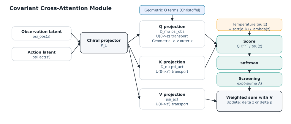
Fig. 8 Covariant cross-attention module. Observation/action latents pass through a chiral projector, then covariant Q/K/V projections with Wilson lines. Scores use temperature \(\tau(z)\) and screening before Values update the state.#
We define the gauge-covariant attention mechanism that respects the full gauge structure.
Definition 282 (Covariant Query-Key-Value Projections)
Let \(\psi_{\text{obs}}(z)\) be the observation latent and \(\psi_{\text{act}}(z')\) be the action latent at positions \(z, z' \in \mathcal{Z}\). The covariant projections are:
where:
\(U_{z \to 0} := U_\gamma(0, z)\) is the Wilson line transporting from \(z\) to the origin (Definition Definition 280)
\(D_\mu\) is the covariant derivative (Definition Definition 279)
\(\Pi_Q, \Pi_K, \Pi_V\) are learnable projection maps that act on feature indices (equivariantly on gauge indices) so they commute with gauge transformations at the reference point
Interpretation:
The Wilson line \(U_{z \to 0}\) parallel-transports the field to a common reference frame at the origin
The covariant derivative \(D_\mu\) ensures the derivative is gauge-covariant
Queries use the derivative \(D_\mu \psi\) (sensitivity to position change)
Values use the field \(\psi\) directly (the actual content to retrieve)
Theorem 98 (Gauge Invariance of Covariant Cross-Attention)
Let the attention score be computed as:
where \(Q\) and \(K\) are defined with Wilson line preprocessing (Definition Definition 282), transporting both to a common reference point (the origin). (If the representation is purely real/orthogonal, replace \(^\dagger\) with transpose and drop \(\operatorname{Re}(\cdot)\).)
Then \(\alpha(z, z')\) is gauge-invariant: under local gauge transformation \(\psi \to \Omega(x)\psi\), the attention score is unchanged.
Proof.
Step 1. Under gauge transformation \(\psi(x) \to \Omega(x)\psi(x)\), the Wilson line transforms as (Definition Definition 280):
Step 2. The covariant derivative transforms covariantly:
Step 3. The Query at \(z\) transforms as:
The \(\Omega^\dagger(z) \Omega(z) = I\) factors cancel:
where the last equality holds because \(\Pi_Q\) acts on feature indices while \(\Omega(0)\) acts on gauge indices (they commute).
Step 4. Similarly, the Key transforms as:
Step 5. The attention score is the inner product at the origin:
The \(\Omega(0)^\dagger \Omega(0) = I\) cancellation occurs because both Q and K have been transported to the same reference point.
Remark (Why no additional Wilson line). Since Q and K are already transported to the origin via Definition Definition 282, their inner product is well-defined without an additional Wilson line. The gauge transformation at the common reference point cancels automatically.
\(\square\)
This theorem is the foundation of the architecture. In the idealized construction, it says that no matter how you choose your local coordinate frames—no matter what gauge you work in—the attention scores come out the same. The Wilson lines act as “gauge correctors” that absorb all the arbitrary choices.
In practice, we approximate the Wilson line for nearby points. For short paths, the path-ordered exponential simplifies to:
This is a linear correction that can be implemented efficiently.
Proposition 97 (Wilson Line Approximation for Attention)
For attention between positions \(z\) and \(z'\) with \(|z - z'| \ll 1\), the Wilson line can be approximated as:
where \(A_\mu\) is the total gauge connection from Definition Definition 280, \(\bar{z}\) is any point along the path (choices differ only at \(O(|z-z'|^2)\)), and the contraction \(A_\mu(\bar{z}) (z - z')^\mu\) is the path-directional connection.
In the attention mechanism, this becomes a relative position encoding:
The second term is the gauge correction to the attention score.
Connection to RL #38: Gauge-Covariant World Models
The General Law (Fragile Agent): World model predictions use covariant cross-attention with Wilson line preprocessing in Q, K, V:
where \(\alpha = \text{softmax}(\operatorname{Re}(Q^\dagger K) / \tau(z_t))\) and Q, K, V include Wilson line transport to a common origin (Definition Definition 282).
The Degenerate Limit: Set all gauge fields to zero (\(G_\mu = W_\mu = B_\mu = 0\)). Wilson lines become identity.
The Special Case (Standard RL): Standard Transformer world models compute:
No gauge structure, no parallel transport, no position-dependent temperature.
What the generalization offers:
Gauge-invariant attention weights (and gauge-covariant outputs) regardless of local gauge choice
Metric-aware temperature scaling for safe exploration
Automatic geodesic correction via geometric (linear + quadratic) Query terms
The Metric in Temperature: Softmax Temperature = Inverse Conformal Factor#
Here is one of the most elegant correspondences in this whole construction. The softmax temperature in attention—that innocuous \(\sqrt{d_k}\) in the denominator—can be made position-dependent and tied directly to the local metric scale.
Think about what temperature does in a softmax. High temperature means soft attention: all positions get similar weight, the distribution is spread out. Low temperature means sharp attention: one position dominates, the distribution is peaked.
Now think about what the metric does in curved space. In high-curvature regions (large metric), distances are “stretched”—small coordinate changes correspond to large proper distances. Motion is difficult. The agent should be cautious, focused, concentrated on nearby states. This is low temperature: sharp attention.
In low-curvature regions (small metric), distances are “compressed”—large coordinate changes correspond to small proper distances. Motion is easy. The agent can explore freely, considering many options. This is high temperature: soft attention.
In a conformal metric \(G(z)=\lambda(z)^2 I\), the conformal factor \(\lambda(z)\) is the local length scale. The simplest monotone choice is therefore: temperature \(\propto 1/\lambda(z)\).
For the Poincare ball/disk, this gives \(\tau(z) = \sqrt{d_k}/\lambda(z) = \sqrt{d_k}(1-|z|^2)/2\). At the origin (where \(|z|=0\)), temperature is \(\sqrt{d_k}/2\) (comparatively soft attention). Near the boundary (as \(|z| \to 1\)), \(\tau(z) \to 0\) and the softmax concentrates on the highest-scoring key.
We derive the position-dependent temperature that encodes the capacity-constrained metric.
Theorem 99 (Metric-Temperature Correspondence)
Let the attention mechanism use position-dependent temperature \(\tau(z)\):
where \(s(z,z')\) is any real-valued score (for example \(s(z,z')=\operatorname{Re}(Q(z)^\dagger K(z'))\)).
The choice
where \(\lambda(z) = 2/(1-|z|^2)\) is the conformal factor, implies:
Metric encoding (conformal case): for \(G(z)=\lambda(z)^2 I\), the metric scale is recovered exactly as \(G(z)=\tfrac{d_k}{\tau(z)^2}I\)
Boundary sharpening: \(\tau(z) \to 0\) as \(|z| \to 1\), so \(\text{softmax}(s/\tau)\) concentrates on the argmax for fixed scores \(s(z,\cdot)\)
Proof.
Step 1 (Metric encoding). For a conformal metric \(G(z)=\lambda(z)^2 I\) and the stated choice of \(\tau(z)\),
so \(G(z)=\tfrac{d_k}{\tau(z)^2}I\) holds identically.
Step 2 (Boundary sharpening). As \(|z| \to 1\):
For any fixed score vector \(s(z,\cdot)\) with a unique maximizer, \(\text{softmax}(s/\tau)\) converges to a point mass on the maximizer as \(\tau\to 0\).
\(\square\)
Proposition 98 (Mass–Metric–Temperature Identity)
The Mass = Metric principle (Definition Definition 67) extends to attention:
Implication (conformal case): Large \(\lambda(z)\) (large metric/mass scale) corresponds to small \(\tau(z)\) (sharper softmax scaling).
This gives us a unified picture. The metric, which encodes capacity and risk, determines three things simultaneously:
How heavy the agent feels (inertial mass)
How sharp the attention is (via \(\tau(z)=\sqrt{d_k}/\lambda(z)\))
How localized the predictions are (attention sharpness)
All from the same geometric quantity. In the conformal case, the identity \(G(z)=\tfrac{d_k}{\tau(z)^2}I\) makes this relationship explicit: temperature is the inverse square root of the metric scale.
Physics Isomorphism: Temperature and Metric
In Physics: In statistical mechanics, the partition function is \(Z = \int e^{-E/k_B T} d\Gamma\). The temperature controls the spread of the Boltzmann distribution. In curved spacetime, the metric affects the integration measure and effective temperature.
In Implementation: The attention mechanism implements:
Correspondence Table:
Statistical Mechanics |
Covariant Attention |
|---|---|
Temperature \(T\) |
Softmax temperature \(\tau(z)\) |
Energy \(E\) |
Negative similarity \(-s(z,z')\) (e.g., \(-\operatorname{Re}(Q^\dagger K)\)) |
Partition function \(Z\) |
Softmax normalizer |
Boltzmann weight \(e^{-E/T}\) |
Attention weight \(\alpha\) |
Metric factor \(\sqrt{g}\) |
Conformal factor \(\lambda(z)^d\) (local scale) |
Christoffel Symbols in Query: Linear + Quadratic Projections for Geodesic Correction#
Now we encode the geodesic correction into the Query projection. This is the most subtle part of the construction.
In the Lorentz-Langevin equation, the Christoffel symbol term is \(-\Gamma^k_{ij} \dot{z}^i \dot{z}^j\). This is quadratic in the velocity. It tells you how much to “curve” your path to stay on the geodesic.
In standard attention, the Query is linear in its input features: \(Q = W_Q x\) (with \(x\) typically encoding \(z\)). This cannot capture the position-dependent connection. We therefore enrich the Query with explicit geometric terms in \(z\) so it can parameterize \(\Gamma(z)\). If you need velocity-conditioned corrections (for discretization residuals or non-Levi-Civita effects), you can add a lightweight bilinear term in \((z, v)\); the core geodesic velocity dependence still comes from the Keys and Values.
What should \(W_{Qz}\) and \(W_{Q,\Gamma}\) be? They should parameterize the Christoffel symbols. The geodesic correction then emerges from the interaction between \(\Gamma(z)\)-aware Queries and velocity-carrying Keys/Values.
The implementation is:
where \(x_v = \phi_v(v)\) is a feature embedding of the current velocity (or momentum). The \(W_{Qz} z\) term captures the linear-in-\(z\) structure of \(\Gamma(z)\) for the Poincare ball/disk, while the \(z \otimes z\) term provides a flexible basis for nonlinear corrections on more general manifolds. The optional \(z \odot v\) term (Hadamard product) provides a simple velocity-conditioned correction when the effective connection departs from the pure Levi-Civita form.
This looks complicated, but the core \(W_{Qz}\) and \(W_{Q,\Gamma}\) terms are the minimum structure needed to encode the geodesic equation; the velocity-conditioned terms are optional corrections. The Christoffel symbols \(\Gamma^k_{ij}\) are symmetric in \(i, j\), and the symmetric outer product \(z \otimes z\) provides a natural basis for that symmetry. The velocity dependence \(\dot{z}^i \dot{z}^j\) comes from the Keys/Values, which encode the action/velocity information.
We derive the geometric (linear + quadratic) Query projection that parameterizes Christoffel symbols for geodesic correction.
Definition 283 (Geodesic Query Projection)
The Geodesic Query extends the linear projection to include geometric terms that encode the Levi-Civita connection (with optional velocity-conditioned corrections when you want to go beyond Levi-Civita):
where:
\(W_Q \in \mathbb{R}^{d_k \times d_{\text{model}}}\) is the feature projection
\(W_{Qz} \in \mathbb{R}^{d_k \times d}\) maps geometric coordinates
\(W_{Qv} \in \mathbb{R}^{d_k \times d_{\text{model}}}\) projects velocity/momentum features \(x_v = \phi_v(v)\)
\(W_{Q,\Gamma} \in \mathbb{R}^{d_k \times d \times d}\) is a 3-tensor encoding position-position quadratic terms
\(W_{Qzv} \in \mathbb{R}^{d_k \times d \times d}\) encodes optional position-velocity coupling
Here \(x_v = \phi_v(v)\) is a feature embedding of velocity/momentum.
Notation: \((A, B)\) denotes bilinear contraction: \(W_{Q,\Gamma}(z, z) = \sum_{ij} W_{Q,\Gamma}^{a,ij} z^i z^j\) and \(W_{Qzv}(z, v) = \sum_{ij} W_{Qzv}^{a,ij} z^i v^j\).
The \(W_{Qzv}\) term is optional; for Levi-Civita connections it can be omitted. In practice, a Hadamard coupling \(z \odot v\) followed by a linear map is often sufficient.
Christoffel Encoding: Use \(W_{Qz}\) to capture the linear-in-\(z\) part of \(\Gamma(z)\) near a reference point \(z_0\), and use \(W_{Q,\Gamma}\) for nonlinear corrections with learnable position dependence. Both can be initialized from the Poincare structure and refined during training.
Theorem 100 (Geodesic Correction Representability via Attention)
Let the Query and Key be:
For clarity, we omit the optional \(W_{Qzv}(z, v)\) term; it adds a velocity-conditioned correction without changing the representability argument.
The attention-weighted output
can represent the geodesic correction term \(-\Gamma^k_{ij}(z) v^i v^j\) when:
The Values include quadratic velocity features (e.g., \(V(z',v') = W_V\,\text{vec}(v' \otimes v')\) or a low-rank factorization)
The Query provides a learned parameterization of the (symmetric) coefficients \(\Gamma(z)\) via the geometric terms (\(W_{Qz}\), \(W_{Q,\Gamma}\))
The context provides velocities in a neighborhood of the current velocity so the quadratic form is sampled/approximated locally
Proof sketch. The attention score is:
With Values containing (symmetrized) quadratic features of \(v'\), an attention-weighted sum can form a linear combination of \(v'^i v'^j\) terms. The geometric Query terms supply position-dependent coefficients, so the module can approximate the contraction \(\Gamma^k_{ij}(z)\,v^i v^j\) up to the approximation induced by softmax and context discretization. \(\square\)
Proposition 99 (Explicit Christoffel Encoding for Poincare Ball/Disk)
For the Poincare ball/disk with Christoffel symbols (Proposition Proposition 19):
A practical initialization is to use a linear geometric term \(W_{Qz} z\) to reproduce the linear-in-\(z\) structure above (up to a sign convention that can be absorbed into the update rule), and reserve \(W_{Q,\Gamma}(z,z)\) for nonlinear corrections. The conformal factor \(2/(1-|z|^2)\) is position-dependent and cannot be represented by a constant \(W_{Qz}\) alone; capture it via \(W_{Q,\Gamma}\) or an explicit scalar modulation.
Learnable approximation: Since \(\Gamma\) depends on position, a simple parameterization is to scale the nonlinear correction by the conformal factor:
where \(\tilde{W}_{Q,\Gamma}\) is a learnable tensor initialized to approximate higher-order corrections and then refined by training.
This is a bit technical, so let me give you the intuition. The Christoffel symbols tell you “when I’m at position \(z\) and moving with velocity \(v\), how much do I need to curve my path to follow the geodesic?” The answer depends on position and quadratically on velocity.
In attention, the Query asks a question and the Key provides answers. The geometric Query terms are asking: “what is the geodesic correction at my current position?” The Key, which contains velocity information, provides the answer through the bilinear interaction.
The nice thing is that this is all learnable. We initialize \(W_{Q,\Gamma}\) with a Poincare-inspired structure, but then let the network fine-tune it based on data. If the Poincare model is exactly right, the network will keep the initialization. If reality is more complex, the network can learn corrections.
\(SU(2)_L\) Chirality: Observation-Action Doublet and Chiral Projector#
Now we implement the chiral structure—the fundamental asymmetry between observation and action.
Recall from the Standard Model of cognition that the left-handed field is a doublet:
This doublet transforms under \(SU(2)_L\), while the right-handed singlet \(\Psi_R = \psi_{\text{act}}^{\text{commit}}\) does not.
In the attention mechanism, we need to preserve this structure. The observation and action channels must be treated as a doublet, with the \(SU(2)\) gauge field mediating their mixing. And the committed action must be extracted via a gauge-covariant projection.
The chiral projector uses the value gradient to define the “direction” of action. Let \(\hat{n}(z)\) be a unit vector in the \(SU(2)\) internal space derived from the value gradient, using a learned projection \(P: \mathbb{R}^d \to \mathbb{R}^3\) when \(d>3\):
where \(\vec{\sigma}\) are the Pauli matrices. The projection operator is:
This projects the doublet onto the component aligned with the value gradient—the direction of improvement.
In flat regions where \(P \nabla V \approx 0\), the projector becomes ambiguous. This is correct: when there is no preferred direction, the agent should not commit to a definite action. The architecture naturally encodes decision ambiguity as projector degeneracy.
We implement the \(SU(2)_L\) gauge structure that distinguishes observation and action channels.
Definition 284 (Observation-Action Doublet in Attention)
The attention mechanism operates on doublet-valued representations:
The Query extracts observation information, the Key encodes action information, both with Wilson line transport to origin (cf. Definition Definition 282):
The cross-attention score between observation and action is (gauge-invariant by Theorem Theorem 98):
Interpretation: The observation at \(z\) attends to actions at \(z'\). Both are transported to a common reference point, ensuring gauge-invariant comparison.
Definition 285 (Chiral Projector from Value Gradient)
The chiral projector extracts committed actions from the observation-action doublet using a unit \(SU(2)\) direction derived from the value gradient:
where \(P: \mathbb{R}^d \to \mathbb{R}^3\) is a learned projection and \(\vec{\sigma} = (\sigma_1, \sigma_2, \sigma_3)\) are Pauli matrices (generators of \(SU(2)\)).
The projection operator is:
The committed action is:
The commitment strength (gauge-invariant under \(SU(2)\), per feature channel) is:
Properties:
\(\Pi_{\text{chirality}}^2 = \Pi_{\text{chirality}}\) (idempotent)
\(\text{Tr}(\Pi_{\text{chirality}}) = 1\) (rank-1 projector)
Under \(SU(2)\) transformation \(\Psi_L \to U\Psi_L\): if \(\hat{n}\) is constructed as an adjoint vector, then \(\hat{n} \to U\hat{n}U^\dagger\), preserving gauge covariance
Degeneracy: When \(\|P \nabla V\| \to 0\) (flat value landscape), \(\hat{n}\) is undefined. The agent should not commit in ambiguous regions.
Theorem 101 (Gauge Covariance of Chiral Projection)
The commitment strength \(c(z) = \Psi_L^\dagger \Pi_{\text{chirality}} \Psi_L\) is invariant under local \(SU(2)_L\) transformations. The projected vector \(\Pi_{\text{chirality}} \Psi_L\) transforms covariantly (in the fundamental representation), but gauge-invariant observables are obtained by contracting the \(SU(2)\) indices.
Proof.
Step 1. Under local \(SU(2)_L\) transformation \(\Psi_L(z) \to U(z)\Psi_L(z)\), where \(U(z) \in SU(2)\).
Step 2. Assume the unit direction \(\hat{n}\) is constructed as an adjoint vector (e.g., via a gauge-covariant map from the value gradient). Then:
Step 3. The projector transforms as:
Step 4. The committed action:
This transforms in the fundamental representation, not as a singlet.
Step 5. To obtain a true singlet, we contract the \(SU(2)\) indices:
This is manifestly gauge-invariant: \(\Psi_L^\dagger U^\dagger \cdot U \Pi U^\dagger \cdot U \Psi_L = \Psi_L^\dagger \Pi \Psi_L\).
\(\square\)
There is a subtlety here that is worth clarifying. The projection \(\Pi \Psi_L\) itself is not a gauge singlet—it still transforms under \(SU(2)\). To get a true invariant, we need to contract the gauge indices (an inner product), not just apply the projector.
In the neural network implementation, we compute a gauge-invariant commitment strength via the inner product \(\Psi_L^\dagger \Pi_{\text{chirality}} \Psi_L\) and use it to gate the projected doublet. If you need a single scalar, you can further sum over feature dimensions.
This has a nice interpretation: the commitment strength is the “correlation” between observation and action intent, weighted by the value gradient direction. High correlation in the gradient direction means strong commitment. Low correlation or ambiguous gradient means weak commitment.
\(SU(N_f)_C\) Texture Firewall: Area Law Screening for Confinement#
The final architectural ingredient is the texture firewall: a screening rule that is intended to prevent raw features from leaking to the macro level. We use confinement language as an analogy for this learned representation constraint.
In QCD, quarks are confined by the strong force. If you try to pull a quark out of a proton, the energy cost grows linearly with distance (the “string” between quarks stretches and stores energy). Eventually it is cheaper to create new quark-antiquark pairs than to keep stretching the string. You never see a free quark.
We want a related behavior for texture. The agent should preferentially observe concepts (bound states of features), rather than raw features. If attention tries to access texture directly, the attention score can be suppressed—screened by an area-law-inspired factor. This is an architectural proxy, not QCD dynamics.
The implementation uses the string tension \(\sigma\) from the binding field (not to be confused with the Pauli matrices \(\sigma^b\) used as \(SU(2)\) generators above). The attention score between positions \(z\) and \(z'\) is modified by:
where \(A_{\text{string}}\) is an area-law-inspired proxy for the cost of coupling distant texture degrees of freedom. In lattice gauge theory, the area law is a statement about closed Wilson loops; here we use a distance-dependent surrogate (typically quadratic in separation) to implement exponential screening in attention.
At the macro level (coarse features), the chosen string-tension schedule can make screening strong. At the texture level (fine features), a smaller schedule can permit texture-to-texture interaction while still limiting the macro path. Calling that schedule “asymptotic freedom” is a physical analogy, not a proved renormalization result.
We implement the \(SU(N_f)_C\) confinement mechanism that screens texture from macro-level access.
Definition 286 (Area Law Screening in Attention)
The screened attention score between positions \(z\) and \(z'\) at representation level \(\ell\) is:
where:
\(\alpha_{\text{bare}}\) is the gauge-covariant attention score from Theorem Theorem 98
\(\sigma(\ell)\) is the string tension at level \(\ell\), with \(\sigma(\ell) \propto g_s^2(\ell)\) (binding coupling squared)
\(A_{\text{string}}(z, z')\) is an area proxy used for screening (often quadratic in separation)
In practice, after applying screening one renormalizes \(\alpha_{\text{screened}}(z,\cdot;\ell)\) over \(z'\) so the weights sum to 1.
Area approximation: For nearby points in flat metric:
For the Poincare ball/disk with conformal factor \(\lambda\):
Theorem 102 (Texture Confinement via Area Law Screening)
Let the representation hierarchy have levels \(\ell = 0\) (macro) to \(\ell = L\) (texture), with running coupling \(g_s(\ell)\) satisfying asymptotic freedom (Definition Definition 256):
Then:
Texture-to-texture attention (\(\ell = L\)): \(\sigma(L) \to 0\), no screening. Features interact freely at texture level.
Macro-to-texture attention (\(\ell = 0\) attending to \(\ell = L\)): \(\sigma(0) > \sigma_{\text{crit}}\), strong screening. Texture is inaccessible from macro level.
Gauge-singlet access: Channels transforming in the trivial (color-neutral) representation of \(SU(N_f)\) can be exempted from screening, allowing macro-level access to bound-state (concept) features while suppressing color-charged texture.
Proof.
Step 1. The string tension is proportional to the coupling squared: \(\sigma(\ell) = c \cdot g_s^2(\ell)\).
Step 2. At texture level, asymptotic freedom gives \(g_s(L) \to 0\), hence \(\sigma(L) \to 0\). The screening factor \(\exp(-\sigma A) \to 1\).
Step 3. At macro level, infrared confinement gives \(g_s(0) > g_s^{\text{crit}}\), hence \(\sigma(0) > \sigma_{\text{crit}}\). For any non-trivial area \(A > 0\), the screening factor \(\exp(-\sigma_{\text{crit}} A) \ll 1\).
Step 4. Gauge-singlet channels do not couple to the binding connection (their generators vanish), so they do not source color flux; equivalently, their effective string tension is zero (or screening is simply not applied on the singlet subspace). Hence the screening factor is 1 on those channels.
\(\square\)
Proposition 100 (Confinement Radius from String Tension)
Assuming the local proxy \(A_{\text{string}}(z,z') \approx d_G(z,z')^2/2\), the confinement radius \(r_{\text{conf}}\) (in geodesic distance) is the scale at which screening suppresses attention by a factor \(e^{-1}\):
At macro level with \(\sigma(0) \approx 1\): \(r_{\text{conf}}(0) \approx \sqrt{2}\) (order-unity in geodesic units).
At texture level with \(\sigma(L) \approx 0.01\): \(r_{\text{conf}}(L) \approx 14\) (large, allowing texture-to-texture interaction).
Interpretation: Weak screening at texture allows long-range texture-to-texture interaction, while strong screening suppresses macro access to color-charged texture channels.
This area-law-inspired screening is a natural architectural proxy for the texture firewall: it implements an exponential suppression of macro-level attention into texture features without requiring hard masks.
And notice that this is not a hard cutoff. The screening is exponential in the chosen area proxy, so nearby texture can influence macro attention weakly, while long-range texture correlations are suppressed when the proxy and coefficient make that estimate valid. The resulting macro independence is an empirical property to test, not a consequence of the QCD analogy.
Physics Isomorphism: Area Law and Confinement
In Physics: In QCD, the potential between quarks grows linearly with distance: \(V(r) = \sigma r\), where \(\sigma \approx 1\) GeV/fm is the string tension. Wilson loops satisfy the area law: \(\langle W(\gamma) \rangle \propto \exp(-\sigma \cdot A)\) where \(A\) is the area enclosed by loop \(\gamma\) [Wilson, 1974].
In Implementation: The screened attention weight is:
Correspondence Table:
QCD |
Covariant Attention |
|---|---|
String tension \(\sigma\) |
Binding coupling squared \(g_s^2\) |
Wilson loop area \(A\) |
String area \(A_{\text{string}}\) |
Quark confinement |
Texture firewall |
Color-neutral hadrons |
Bound-state concepts \(K\) |
Asymptotic freedom |
Texture-level weak coupling |
BAOAB Integration via Attention Heads and OU Thermostat#
Now we put it all together. The Boris-BAOAB integrator has five steps: B-A-O-A-B. We implement the B and A steps as attention heads, and the O-step as a closed-form OU update by default (with an optional learned thermostat head when you want richer noise).
Why five steps? Because each part of BAOAB does something different:
B (kick): Apply forces from the potential gradient
A (drift): Move along the geodesic
O (thermostat): Add thermal noise
A (drift): Continue moving
B (kick): Apply more forces
Each step needs to attend to different information. The kick steps need the potential gradient (stored in Keys). The drift steps use the explicit velocity \(v = G^{-1}p\) and can add attention-based displacement corrections from Values. The thermostat step injects OU noise directly, with an optional learned residual if you enable the O-head.
The Keys act as a “gradient bank.” They store the gradients of the effective potential at various positions. When the Query asks “what force do I feel here?”, the Key provides the answer through the attention score.
The Values act as “state updates.” After computing the attention weights, the weighted sum of Values gives a correction update to position or momentum (added to the explicit drift or OU step).
The temperature of each head is position-dependent, encoding the metric. And the Wilson lines ensure gauge covariance throughout.
The result is a single attention block with four heads (or five if you enable the learned thermostat) that performs one complete step of the geodesic integrator. Stack multiple blocks for multi-step rollouts.
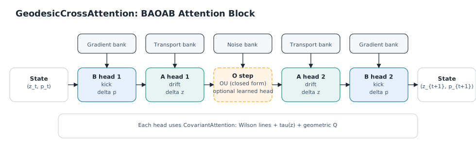
Fig. 9 BAOAB attention block. Four covariant attention heads implement B-A-O-A-B around an OU thermostat, producing one integrator step from \((z_t, p_t)\) to \((z_{t+1}, p_{t+1})\).#
We implement the Boris-BAOAB integrator (Definition Definition 74) using four specialized attention heads plus a closed-form OU thermostat (or five heads if you enable a learned thermostat).
Definition 287 (BAOAB Steps (Attention Heads + OU))
The GeodesicCrossAttention module implements B-A-O-A-B with attention heads for B/A and a closed-form OU step in the middle (or an optional learned O-head):
Step 1 (B-head 1): B-step (First half-kick)
Query: Current position \(z\) with quadratic geodesic terms
Key: Gradient bank \(\{\nabla\Phi(z')\}_{z' \in \text{context}}\)
Value: Gradient vectors \(\{\nabla\Phi(z')\}\)
Output: Momentum update \(\Delta p_1 = -\frac{h}{2}\nabla\Phi(z)\)
Step 2 (A-head 1): A-step (First half-drift)
Query: Current position and momentum \((z, p)\)
Key: Exponential map or transport bank \(\{\exp_{z'}(v)\}\)
Value: Displacement corrections
Output: Drift correction \(\Delta z_1\) added to the explicit drift \(\frac{h}{2}G^{-1}(z)p\)
Step 3 (OU): O-step (Ornstein-Uhlenbeck thermostat)
Default: Closed-form OU update (no attention)
Optional learned thermostat:
Query: Current momentum \(p\)
Key: Noise bank (random vectors)
Value: Noise vectors \(\{\xi\}\)
Output: Residual correction added to the OU update
Step 4 (A-head 2): A-step (Second half-drift)
Same structure as Step 2
Output: Drift correction \(\Delta z_2\) added to the explicit drift \(\frac{h}{2}G^{-1}(z)p\)
Step 5 (B-head 2): B-step (Second half-kick)
Same structure as Step 1
Output: Momentum update \(\Delta p_2 = -\frac{h}{2}\nabla\Phi(z)\)
Composition: The full update is:
Here \(\text{Step}_3\) denotes the OU operator unless a learned thermostat head is enabled.
Theorem 103 (BAOAB Attention Targets Boltzmann Distribution (Idealized))
In the idealized setting where the attention heads recover the BAOAB substeps (kick/drift) and the O-step is the exact OU update, the GeodesicCrossAttention module reduces to the standard BAOAB integrator (Definition Definition 74). In that limit, it targets the Gibbs/Boltzmann density
as the intended stationary distribution (cf. Proposition Proposition 21), provided:
Each head uses position-dependent temperature \(\tau(z) = \sqrt{d_k}/\lambda(z)\)
The O-step uses thermalization coefficients \(c_1 = e^{-\gamma h}\), \(c_2 = \sqrt{(1-c_1^2)T_c}\)
The geodesic Query projections correctly encode Christoffel symbols
The A-steps include the explicit drift \(G^{-1}(z)p\) (with any attention-based correction consistent with the exponential map)
Proof sketch. This follows from Proposition Proposition 21 applied to the attention implementation. The key points:
The symmetric splitting B-A-O-A-B ensures time-reversibility of deterministic steps.
The A-steps include the explicit drift \(G^{-1}p\), with attention providing higher-order corrections.
The O-step is an exact OU transition, which leaves the Maxwell-Boltzmann conditional momentum distribution invariant (for fixed \(z\) and the chosen mass tensor).
Position-dependent temperature correctly weights attention by the metric.
Wilson lines preserve gauge covariance without affecting thermodynamic properties.
If a learned thermostat head is enabled, the O-step becomes a data-driven approximation that may deviate from exact OU sampling; treat this as a controlled modeling choice and monitor with diagnostic checks. Likewise, attention-based interpolation of gradients, drift corrections, and Wilson lines introduces additional approximation error beyond the baseline BAOAB discretization. \(\square\)
Experiment: Thermostat Ablation
Compare the exact OU thermostat (no O-head) against a learned thermostat residual (diffusion-style noise). Track (i) momentum marginal vs. Maxwell-Boltzmann, (ii) energy drift over long rollouts, (iii) Node 68 metric-temperature consistency, and (iv) forecast accuracy or sample efficiency. This isolates expressivity vs. thermodynamic fidelity.
Proposition 101 (Keys as Gradient Bank)
In the B-step attention heads, the Keys store precomputed gradients of the effective potential at context positions:
The attention score \(s(z, z') := \operatorname{Re}\left(Q(z)^\dagger K(z')\right)\) measures how aligned the current position is with the gradient at \(z'\). The weighted sum of Values retrieves the local gradient estimate:
The B-step applies the negative sign: \(\Delta p = -\frac{h}{2}\widehat{\nabla\Phi}(z)\).
Advantage: Precomputing gradients at context positions amortizes the cost of gradient computation across multiple queries.
Proposition 102 (Values as State Updates)
In each attention head, the Values encode the update to apply (the OU step is closed-form unless you enable a learned thermostat):
Head |
Value Content |
Update |
|---|---|---|
B (kick) |
\(\nabla\Phi\) |
\(\Delta p\) (with negative sign applied in the update) |
A (drift) |
Displacement correction |
\(\Delta z\) (added to explicit \(G^{-1}p\) drift) |
O (thermostat) |
\(c_2\,G^{1/2}\xi\) (OU) |
Noise injection (optional learned residual) |
The attention-weighted Value sum produces the correction update, which is added to the explicit drift or momentum update as appropriate.
Implementation: Full GeodesicCrossAttention Module#
Here is the complete implementation. It looks like a lot of code, but each piece corresponds directly to something we have derived mathematically.
The main class GeodesicCrossAttention has four attention heads for the B and A steps, plus an optional learned thermostat head. Each attention head uses the CovariantAttention helper class, which handles Wilson lines, position-dependent temperature, and geometric (linear + quadratic) Query projections.
The forward method takes the current state \((z, p)\) along with context banks (forces for B-steps, drift corrections for A-steps) and produces the next state \((z', p')\) in one pass. Inside, it sequences through the five BAOAB steps: kick, drift, thermostat, drift, kick, using four attention heads by default and a closed-form OU step for the thermostat. Because attention operates in \(d_{\text{model}}\), the head outputs are projected back to \(d_{\text{latent}}\) before applying updates when the dimensions differ.
Pay attention to the metric computation. We use the Poincare ball/disk formula, but this is modular—you can swap in any other metric by changing the conformal_factor method.
The Wilson line approximation uses the linearized form for nearby points. For long-range attention, you would need to accumulate the path-ordered product, which is more expensive.
The Christoffel symbols are encoded in the geometric Query projection. The linear term W_Qz and the tensor W_Q_gamma can be initialized with a Poincare-inspired pattern, but they are learnable.
We provide a PyTorch implementation of the GeodesicCrossAttention module. This is demonstrative code illustrating the architecture; a production implementation would require additional numerical care.
Implementation Note
The code below is a prototype implementation intended to illustrate the architecture’s structure. For production use, several enhancements are needed:
Wilson lines: The linear approximation is valid only for nearby points. Long-range attention requires path-ordered products or geodesic interpolation.
Christoffel initialization: The linear (\(W_{Qz}\)) and quadratic (\(W_{Q,\Gamma}\)) terms should be initialized more carefully if you want an exact Poincare match.
Numerical stability: Additional clamping and normalization may be needed near the boundary where \(\lambda \to \infty\).
Chiral projector: The SU(2) structure uses a real-valued proxy; a full implementation should use complex Pauli matrices and an explicit adjoint mapping for \(\hat{n}\).
Head-specific inputs: In production, use distinct Key/Value banks per head (forces for B, transport corrections for A, noise for optional learned O). The prototype uses
context_forcefor B and reusescontext_xfor A.Thermostat choice: The default OU step is exact. If you enable a learned thermostat head, treat it as a residual correction and monitor distributional drift.
State updates: If \(d_{\text{model}} \neq d_{\text{latent}}\), project attention outputs back to latent coordinates before applying updates.
Implementation vs. Theory: The mathematical formulation (Definition Definition 282) has Wilson lines embedded in Q, K, V definitions. The code uses an equivalent decomposition in the idealized setting: Wilson line correction is applied at attention-time via K_transported = U @ K. With approximate Wilson lines, gauge invariance becomes approximate and should be monitored (Node 67).
The essential mathematical structure is preserved: Wilson line preprocessing, position-dependent temperature, geometric Query, and BAOAB splitting.
"""
GeodesicCrossAttention: Gauge-covariant world model as geodesic integrator.

Cross-references:
    - Definition {prf:ref}`def-covariant-qkv-projections` (Covariant Q/K/V)
    - Theorem {prf:ref}`thm-gauge-invariance-cross-attention` (Gauge invariance)
    - Theorem {prf:ref}`thm-metric-temperature-correspondence` (Metric-temperature)
    - Definition {prf:ref}`def-baoab-attention-heads` (BAOAB steps)
"""

import torch
import torch.nn as nn
import torch.nn.functional as F
import math
from dataclasses import dataclass
from typing import Tuple, Optional


@dataclass
class GeodesicConfig:
    """Configuration for GeodesicCrossAttention.

    Args:
        d_model: Model dimension [nat]
        d_latent: Latent space dimension
        n_heads: Number of attention heads per BAOAB step (default: 1)
        T_c: Cognitive temperature [nat/step]
        gamma_friction: Friction coefficient for O-step
        dt: Integration timestep
        g_s: Binding coupling strength (for area law screening)
        g_2: Error field coupling (for SU(2) chirality)
        g_1: Opportunity field coupling (for U(1) hypercharge)
        use_learned_thermostat: Enable learned thermostat residual (optional)
        thermostat_residual_scale: Scale for learned thermostat residual
    """
    d_model: int = 256
    d_latent: int = 64
    n_heads: int = 1
    T_c: float = 0.1
    gamma_friction: float = 1.0
    dt: float = 0.01
    g_s: float = 1.0
    g_2: float = 0.5
    g_1: float = 0.3
    use_learned_thermostat: bool = False
    thermostat_residual_scale: float = 0.1


class WilsonLineApprox(nn.Module):
    """
    Approximate Wilson line for parallel transport.

    Real/orthogonal proxy for the first-order Wilson line:
        U(z, z') ≈ I + H(Δz)

    where H(Δz) is skew-symmetric and represents (-i A·Δz) in a real-valued
    implementation.

    Cross-reference: Proposition {prf:ref}`prop-wilson-line-approximation`
    """

    def __init__(self, config: GeodesicConfig, d_k: int, d_conn: int = 8):
        super().__init__()
        self.d_k = d_k
        self.d_conn = min(d_conn, config.d_latent)

        # Project latent displacements into a low-dimensional coefficient vector
        self.delta_proj = nn.Linear(config.d_latent, self.d_conn, bias=False)

        # Skew-symmetric basis matrices for each gauge factor (proxy)
        self.basis_binding = nn.Parameter(0.01 * torch.randn(self.d_conn, d_k, d_k))
        self.basis_error = nn.Parameter(0.01 * torch.randn(self.d_conn, d_k, d_k))
        self.basis_opportunity = nn.Parameter(0.01 * torch.randn(self.d_conn, d_k, d_k))

        self.g_s = config.g_s
        self.g_2 = config.g_2
        self.g_1 = config.g_1

    def forward(
        self,
        z_query: torch.Tensor,  # [B, d_latent]
        z_key: torch.Tensor,    # [B, N, d_latent]
    ) -> torch.Tensor:
        """
        Compute Wilson line correction factor.

        Returns: [B, N, d_k, d_k] transformation matrix for each key position.
        """
        B, N, _ = z_key.shape

        # Displacement z - z'
        delta_z = z_query.unsqueeze(1) - z_key  # [B, N, d_latent]
        coeff = self.delta_proj(delta_z)  # [B, N, d_conn]

        def skew(basis: torch.Tensor) -> torch.Tensor:
            return basis - basis.transpose(-1, -2)

        H = (
            self.g_s * torch.einsum('bnr,rij->bnij', coeff, skew(self.basis_binding))
            + self.g_2 * torch.einsum('bnr,rij->bnij', coeff, skew(self.basis_error))
            + self.g_1 * torch.einsum('bnr,rij->bnij', coeff, skew(self.basis_opportunity))
        )  # [B, N, d_k, d_k]

        # First-order approximation: U ≈ I + H.
        # For a group element, use torch.matrix_exp(H) (more expensive).
        d_k = self.d_k
        identity = torch.eye(d_k, device=z_key.device, dtype=z_key.dtype).expand(B, N, d_k, d_k)
        return identity + H  # [B, N, d_k, d_k]


class ConformalMetric(nn.Module):
    """
    Poincare ball/disk metric computations.

    λ(z) = 2 / (1 - |z|²)
    G_ij = λ² δ_ij

    Cross-reference: Definition {prf:ref}`def-poincare-metric-recap`
    """

    def __init__(self, epsilon: float = 1e-6):
        super().__init__()
        self.epsilon = epsilon

    def conformal_factor(self, z: torch.Tensor) -> torch.Tensor:
        """
        Compute conformal factor λ(z) = 2 / (1 - |z|²).

        Args:
            z: [B, d] positions in Poincare ball/disk

        Returns: [B, 1] conformal factors
        """
        r_sq = (z ** 2).sum(dim=-1, keepdim=True)
        # Clamp to ensure we stay inside disk
        r_sq = torch.clamp(r_sq, max=1.0 - self.epsilon)
        lambda_z = 2.0 / (1.0 - r_sq + self.epsilon)
        return lambda_z

    def metric(self, z: torch.Tensor) -> torch.Tensor:
        """
        Compute metric tensor G_ij(z).

        Returns: [B, d, d] metric tensors
        """
        B, d = z.shape
        lambda_sq = self.conformal_factor(z) ** 2  # [B, 1]
        return lambda_sq.unsqueeze(-1) * torch.eye(d, device=z.device, dtype=z.dtype)

    def metric_inv(self, z: torch.Tensor) -> torch.Tensor:
        """
        Compute inverse metric G^{ij}(z).

        Returns: [B, d, d] inverse metric tensors
        """
        B, d = z.shape
        lambda_sq_inv = 1.0 / (self.conformal_factor(z) ** 2 + self.epsilon)
        return lambda_sq_inv.unsqueeze(-1) * torch.eye(d, device=z.device, dtype=z.dtype)

    def temperature(self, z: torch.Tensor, d_k: int) -> torch.Tensor:
        """
        Position-dependent attention temperature.

        τ(z) = √d_k / λ(z)

        Cross-reference: Theorem {prf:ref}`thm-metric-temperature-correspondence`

        Returns: [B, 1] temperatures
        """
        lambda_z = self.conformal_factor(z)
        return math.sqrt(d_k) / lambda_z


class ChristoffelQuery(nn.Module):
    """
    Geometric Query projection encoding Christoffel symbols.

    Q(x, z, v) = W_Q x + W_Qz z + W_Qv v_feat + W_QΓ(z, z) + W_Qzv(z, v)

    Cross-reference: Definition {prf:ref}`def-geodesic-query-projection`
    """

    def __init__(self, d_in: int, d_out: int, d_latent: int):
        super().__init__()

        # Linear projections
        self.W_Q = nn.Linear(d_in, d_out, bias=False)
        self.W_Qz = nn.Linear(d_latent, d_out, bias=False)
        self.W_Qv = nn.Linear(d_in, d_out, bias=False)

        # Quadratic projection (3-tensor for Christoffel encoding)
        # Initialized with a Poincare-inspired pattern
        self.W_Q_gamma = nn.Parameter(torch.zeros(d_out, d_latent, d_latent))
        self._init_christoffel(d_latent)

        # Position-velocity coupling
        self.W_Qzv = nn.Parameter(torch.zeros(d_out, d_latent, d_latent))

    def _init_christoffel(self, d: int):
        """Initialize W_Q_gamma to approximate Poincare Christoffel structure."""
        # Γ^k_ij ∝ (δ^k_i z_j + δ^k_j z_i - δ_ij z^k)
        # We initialize with small random values; exact structure is learned
        with torch.no_grad():
            for k in range(min(d, self.W_Q_gamma.shape[0])):
                for i in range(d):
                    for j in range(d):
                        if i == k or j == k:
                            self.W_Q_gamma[k, i, j] = 0.01
                        if i == j:
                            self.W_Q_gamma[k, i, j] -= 0.01

    def forward(
        self,
        x: torch.Tensor,        # [B, d_in] feature vector
        z_geom: torch.Tensor,   # [B, d_latent] position
        v_feat: Optional[torch.Tensor] = None,  # [B, d_in] velocity features
        v_geom: Optional[torch.Tensor] = None,  # [B, d_latent] velocity
    ) -> torch.Tensor:
        """
        Compute geodesic Query.

        Returns: [B, d_out] Query vectors
        """
        # Linear terms
        Q = self.W_Q(x) + self.W_Qz(z_geom)  # [B, d_out]

        # Velocity term (if provided)
        if v_feat is not None:
            Q = Q + self.W_Qv(v_feat)

        # Quadratic term (Christoffel encoding)
        # W_QΓ(z, z) = sum_ij W_QΓ^a_ij z^i z^j
        d = min(z_geom.shape[-1], self.W_Q_gamma.shape[-1])
        z_trunc = z_geom[..., :d]
        Q_gamma = torch.einsum('aij,bi,bj->ba', self.W_Q_gamma[:, :d, :d], z_trunc, z_trunc)
        Q = Q + Q_gamma

        # Position-velocity coupling (if velocity provided)
        if v_geom is not None:
            v_trunc = v_geom[..., :d]
            Q_zv = torch.einsum('aij,bi,bj->ba', self.W_Qzv[:, :d, :d], z_trunc, v_trunc)
            Q = Q + Q_zv

        return Q


class ChiralProjector(nn.Module):
    """
    SU(2)_L chiral projector from value gradient.

    Π = (1/2)(I + n·σ) where n = proj(∇V) / ||proj(∇V)||

    Cross-reference: Definition {prf:ref}`def-chiral-projector-value-gradient`
    """

    def __init__(self, d_latent: int):
        super().__init__()
        self.d_latent = d_latent

        # Project gradient into SU(2) direction
        self.grad_proj = nn.Linear(d_latent, 3, bias=False)

        # Pauli matrices (real-valued proxy for 2x2 case)
        # Note: σ_2 is purely imaginary in the standard complex representation;
        # we use (-i σ_2) as a real proxy here.
        self.register_buffer('identity', torch.eye(2))
        self.register_buffer('sigma_1', torch.tensor([[0., 1.], [1., 0.]]))
        self.register_buffer('sigma_2', torch.tensor([[0., -1.], [1., 0.]]))
        self.register_buffer('sigma_3', torch.tensor([[1., 0.], [0., -1.]]))

    def forward(
        self,
        psi_doublet: torch.Tensor,  # [B, 2, d] observation-action doublet
        grad_V: torch.Tensor,        # [B, d_latent] value gradient
    ) -> torch.Tensor:
        """
        Apply chiral projection and compute commitment strength.

        Returns: [B, 2*d] gated projected doublet (commitment strength from Ψ†ΠΨ)
        """
        # Project and normalize gradient to get SU(2) direction
        n = self.grad_proj(grad_V)  # [B, 3]
        n = n / (torch.norm(n, dim=-1, keepdim=True) + 1e-8)
        n_x, n_y, n_z = n.unbind(dim=-1)

        # Build projector Π = (1/2)(I + n·σ)
        proj = 0.5 * (
            self.identity
            + n_x[:, None, None] * self.sigma_1
            + n_y[:, None, None] * self.sigma_2
            + n_z[:, None, None] * self.sigma_3
        )

        # Apply projector and compute gauge-invariant commitment strength
        psi_proj = torch.einsum('bij,bjd->bid', proj, psi_doublet)  # [B, 2, d]
        # For complex fields, replace with (psi_doublet.conj() * psi_proj).sum(...)
        commit_strength = (psi_doublet * psi_proj).sum(dim=1, keepdim=True)  # [B, 1, d]
        psi_proj = psi_proj * commit_strength
        return psi_proj.reshape(psi_proj.shape[0], -1)  # [B, 2*d]


class AreaLawScreening(nn.Module):
    """
    SU(N_f)_C area law screening for texture confinement.

    Applied to attention weights (after softmax):
        α_screened = α · exp(-σ · A_string)

    The output is then renormalized to sum to 1.

    Cross-reference: Definition {prf:ref}`def-area-law-screening-attention`
    """

    def __init__(self, config: GeodesicConfig):
        super().__init__()
        self.g_s = config.g_s

        # String tension (learnable, initialized from coupling)
        self.log_sigma = nn.Parameter(torch.log(torch.tensor(config.g_s ** 2)))

    @property
    def sigma(self) -> torch.Tensor:
        return torch.exp(self.log_sigma)

    def string_area(
        self,
        z_query: torch.Tensor,  # [B, d]
        z_key: torch.Tensor,    # [B, N, d]
        lambda_z: torch.Tensor,  # [B, 1] conformal factor at query
    ) -> torch.Tensor:
        """
        Compute string-area proxy between positions.

        A ≈ (λ²/2) |z - z'|²

        Returns: [B, N] string areas
        """
        delta_z = z_query.unsqueeze(1) - z_key  # [B, N, d]
        dist_sq = (delta_z ** 2).sum(dim=-1)  # [B, N]
        area = 0.5 * (lambda_z ** 2) * dist_sq
        return area

    def forward(
        self,
        attention: torch.Tensor,  # [B, N] attention scores
        z_query: torch.Tensor,
        z_key: torch.Tensor,
        lambda_z: torch.Tensor,
        level: int = 0,  # hierarchy level (0=macro, L=texture)
    ) -> torch.Tensor:
        """
        Apply area law screening to attention.

        Returns: [B, N] screened attention
        """
        area = self.string_area(z_query, z_key, lambda_z)

        # Level-dependent coupling (asymptotic freedom)
        # σ(ℓ) = σ_0 · exp(-ℓ / L) for UV decay
        L_max = 10  # maximum hierarchy depth
        sigma_eff = self.sigma * math.exp(-level / L_max)

        # Screening factor
        screening = torch.exp(-sigma_eff * area)

        return attention * screening


class CovariantAttention(nn.Module):
    """
    Single covariant attention head with all gauge structures.

    Combines:
        - Wilson line preprocessing
        - Position-dependent temperature
        - Geometric Query (Christoffel)
        - Chiral projection (optional)
        - Area law screening (optional)
    """

    def __init__(
        self,
        config: GeodesicConfig,
        use_chirality: bool = False,
        use_screening: bool = False,
        head_type: str = 'generic',  # 'B', 'A', 'O', or 'generic'
    ):
        super().__init__()
        self.config = config
        self.use_chirality = use_chirality
        self.use_screening = use_screening
        self.head_type = head_type

        d = config.d_model
        d_k = d // config.n_heads

        # Core projections
        self.query = ChristoffelQuery(d, d_k, config.d_latent)
        self.key = nn.Linear(d, d_k, bias=False)
        self.value = nn.Linear(d, d_k, bias=False)
        self.output = nn.Linear(d_k, d, bias=False)

        # Gauge structures
        self.wilson = WilsonLineApprox(config, d_k)
        self.metric = ConformalMetric()

        if use_chirality:
            self.chiral = ChiralProjector(config.d_latent)

        if use_screening:
            self.screening = AreaLawScreening(config)

        self.d_k = d_k

    def forward(
        self,
        z_query: torch.Tensor,     # [B, d_latent] query position
        z_key: torch.Tensor,       # [B, N, d_latent] key positions
        x_query: torch.Tensor,     # [B, d_model] query features
        x_key: torch.Tensor,       # [B, N, d_model] key features
        x_value: torch.Tensor,     # [B, N, d_model] value features
        v_query: Optional[torch.Tensor] = None,  # [B, d_model] velocity features
        v_query_geom: Optional[torch.Tensor] = None,  # [B, d_latent] velocity
        grad_V: Optional[torch.Tensor] = None,   # [B, d_latent] value gradient
        level: int = 0,
    ) -> Tuple[torch.Tensor, torch.Tensor]:
        """
        Compute covariant attention.

        Returns:
            output: [B, d_model] attention output
            attention: [B, N] attention weights
        """
        B, N, _ = x_key.shape

        # Compute Q, K, V with geodesic Query
        Q = self.query(x_query, z_query, v_query, v_query_geom)  # [B, d_k]
        K = self.key(x_key)                # [B, N, d_k]
        V = self.value(x_value)            # [B, N, d_k]

        # Wilson line correction to Keys
        U = self.wilson(z_query, z_key)  # [B, N, d_k, d_k] (approx)
        K_transported = torch.einsum('bnij,bnj->bni', U, K)

        # Attention scores with Wilson-corrected Keys
        scores = torch.einsum('bi,bni->bn', Q, K_transported)  # [B, N]

        # Position-dependent temperature
        tau = self.metric.temperature(z_query, self.d_k)  # [B, 1]
        scores = scores / (tau + 1e-8)

        # Softmax
        attention = F.softmax(scores, dim=-1)  # [B, N]

        # Area law screening (if enabled) - applied after softmax per Definition
        if self.use_screening:
            lambda_z = self.metric.conformal_factor(z_query)
            attention = self.screening(attention, z_query, z_key, lambda_z, level)
            # Renormalize after screening
            attention = attention / (attention.sum(dim=-1, keepdim=True) + 1e-8)

        # Weighted sum of Values
        output = torch.einsum('bn,bni->bi', attention, V)  # [B, d_k]

        # Chiral projection (if enabled and gradient provided)
        if self.use_chirality and grad_V is not None:
            if output.shape[-1] % 2 != 0:
                raise ValueError("Chiral projection requires an even d_k.")
            # Reshape output as doublet for projection
            output_doublet = output.reshape(B, 2, -1)
            output = self.chiral(output_doublet, grad_V)
            output = output.reshape(B, -1)

        # Output projection
        output = self.output(output)

        return output, attention


class GeodesicCrossAttention(nn.Module):
    """
    Full geodesic world model implementing Boris-BAOAB integration.

    Four attention heads for B-A-A-B, with an optional learned thermostat head.

    Cross-reference: Definition {prf:ref}`def-baoab-attention-heads`

    Usage:
        model = GeodesicCrossAttention(config)
        z_next, p_next = model(z, p, context_z, context_x, context_force)
    """

    def __init__(self, config: GeodesicConfig):
        super().__init__()
        self.config = config

        # BAOAB coefficients
        self.dt = config.dt
        self.gamma = config.gamma_friction
        self.T_c = config.T_c
        self.c1 = math.exp(-self.gamma * self.dt)
        self.c2 = math.sqrt((1 - self.c1 ** 2) * self.T_c) if self.T_c > 0 else 0.0

        # Metric computations
        self.metric = ConformalMetric()

        # BAOAB attention heads (B, A, A, B) plus optional learned thermostat
        self.head_B1 = CovariantAttention(config, head_type='B')
        self.head_A1 = CovariantAttention(config, head_type='A')
        self.use_learned_thermostat = config.use_learned_thermostat
        self.thermostat_residual_scale = config.thermostat_residual_scale
        if self.use_learned_thermostat:
            self.head_O = CovariantAttention(config, head_type='O')
        else:
            self.head_O = None
        self.head_A2 = CovariantAttention(config, head_type='A')
        self.head_B2 = CovariantAttention(config, head_type='B')

        # Encoders for geometry, forces, and velocities
        self.pos_encoder = nn.Linear(config.d_latent, config.d_model)
        self.grad_encoder = nn.Linear(config.d_latent, config.d_model)
        self.velocity_encoder = nn.Linear(config.d_latent, config.d_model)

        # Project attention outputs back to latent updates
        self.state_proj = nn.Linear(config.d_model, config.d_latent)

        # Noise projection for optional learned thermostat
        if self.use_learned_thermostat:
            self.noise_proj = nn.Linear(config.d_latent, config.d_model)
        else:
            self.noise_proj = None

    def forward(
        self,
        z: torch.Tensor,           # [B, d_latent] current position
        p: torch.Tensor,           # [B, d_latent] current momentum
        context_z: torch.Tensor,   # [B, N, d_latent] context positions
        context_x: torch.Tensor,   # [B, N, d_model] context features (drift corrections)
        context_force: torch.Tensor,  # [B, N, d_latent] force/gradient bank
    ) -> Tuple[torch.Tensor, torch.Tensor]:
        """
        One step of geodesic BAOAB integration.

        Returns:
            z_next: [B, d_latent] updated position
            p_next: [B, d_latent] updated momentum
        """
        h = self.dt

        # Encode force bank
        force_features = self.grad_encoder(context_force)

        # ===== B-step 1: First half-kick =====
        delta_p1, _ = self.head_B1(
            z_query=z,
            z_key=context_z,
            x_query=self.pos_encoder(z),
            x_key=force_features,
            x_value=force_features,
        )
        # Interpret as momentum update
        delta_p1_latent = self.state_proj(delta_p1)
        p = p - (h / 2) * delta_p1_latent

        # ===== A-step 1: First half-drift =====
        # Compute velocity from momentum
        G_inv = self.metric.metric_inv(z)
        v = torch.einsum('bij,bj->bi', G_inv, p)

        delta_z1, _ = self.head_A1(
            z_query=z,
            z_key=context_z,
            x_query=self.pos_encoder(z) + self.velocity_encoder(v),
            x_key=context_x,
            x_value=context_x,
            v_query=self.velocity_encoder(v),
            v_query_geom=v,
        )
        # Apply position update via exponential map approximation
        delta_z1_latent = self.state_proj(delta_z1)
        z = z + (h / 2) * (v + delta_z1_latent)
        z = self._project_to_disk(z)

        # ===== O-step: Ornstein-Uhlenbeck thermostat =====
        # Thermalize momentum (closed-form OU)
        G_sqrt = self.metric.conformal_factor(z)
        xi = torch.randn_like(p)
        p = self.c1 * p + self.c2 * G_sqrt * xi
        # Optional learned thermostat residual (diffusion-style correction)
        if self.use_learned_thermostat:
            noise_bank = torch.randn_like(context_z)
            noise_features = self.noise_proj(noise_bank)
            delta_p_noise, _ = self.head_O(
                z_query=z,
                z_key=context_z,
                x_query=self.velocity_encoder(p),
                x_key=noise_features,
                x_value=noise_features,
            )
            delta_p_noise_latent = self.state_proj(delta_p_noise)
            p = p + self.thermostat_residual_scale * delta_p_noise_latent

        # ===== A-step 2: Second half-drift =====
        G_inv = self.metric.metric_inv(z)
        v = torch.einsum('bij,bj->bi', G_inv, p)

        delta_z2, _ = self.head_A2(
            z_query=z,
            z_key=context_z,
            x_query=self.pos_encoder(z) + self.velocity_encoder(v),
            x_key=context_x,
            x_value=context_x,
            v_query=self.velocity_encoder(v),
            v_query_geom=v,
        )
        delta_z2_latent = self.state_proj(delta_z2)
        z = z + (h / 2) * (v + delta_z2_latent)
        z = self._project_to_disk(z)

        # ===== B-step 2: Second half-kick =====
        delta_p2, _ = self.head_B2(
            z_query=z,
            z_key=context_z,
            x_query=self.pos_encoder(z),
            x_key=force_features,
            x_value=force_features,
        )
        delta_p2_latent = self.state_proj(delta_p2)
        p = p - (h / 2) * delta_p2_latent

        return z, p

    def _project_to_disk(self, z: torch.Tensor, max_norm: float = 0.999) -> torch.Tensor:
        """Project z to interior of Poincare ball/disk."""
        norm = torch.norm(z, dim=-1, keepdim=True)
        return torch.where(norm > max_norm, z * max_norm / norm, z)
A few notes on the implementation:
Efficiency: The Wilson line computation is the most expensive part. In practice, you would precompute it for the context positions and cache it across heads.
Initialization: The linear term \(W_{Qz}\) and the Christoffel tensor \(W_{Q,\Gamma}\) can be initialized with a Poincare-inspired pattern. During training, they can adapt to the actual geometry of the learned latent space.
Stability: The projection to disk at the end of each step ensures we never leave the representable region. This is a safety net on top of the geometric constraints.
Modularity: Each component (Wilson lines, metric, Christoffel, chirality, screening) is a separate module. You can enable or disable them independently depending on which gauge structures you need.
Computational Complexity and O(N) Engineering Proxies#
Now let me address the elephant in the room: computational complexity. The architecture I have described is beautiful mathematically, but if you implement it naively, it will be slow. Very slow.
The problem is that attention is inherently \(O(N^2)\)—every query attends to every key. On top of that, we have added Wilson lines, which require path integrals. And quadratic/bilinear Query terms, which add \(O(d^2)\) parameters. And area law screening, which requires computing string areas for every pair.
For a context of \(N = 1000\) positions and latent dimension \(d = 64\), the naive complexity is \(O(N^2 d^2) \approx 4 \times 10^9\) operations per attention layer. That is not practical.
But here is the useful engineering possibility: under an explicit decay estimate for the chosen screening proxy, we can approximate the interaction with \(O(N)\) or \(O(N \log N)\) sparse patterns while controlling the discarded tail. Gauge covariance is a local identity, but locality alone does not supply a complexity bound; the Wilson-line and screening errors must be measured.
Let me show you how to do this systematically.
The naive implementation of covariant cross-attention has complexity \(O(N^2 d^2)\) per layer. We derive practical approximations that achieve \(O(N)\) or \(O(N \log N)\) complexity while preserving the essential gauge structure.
Proposition 103 (Complexity of Naive Implementation)
The full covariant cross-attention has the following complexity breakdown:
Component |
Naive Complexity |
Bottleneck |
|---|---|---|
Wilson line computation |
\(O(N^2 d^2)\) |
Path integral for each pair |
Attention scores |
\(O(N^2 d)\) |
All-pairs dot product |
Quadratic Query |
\(O(N d^2)\) |
Christoffel tensor contraction |
Area law screening |
\(O(N^2)\) |
String area for each pair |
Chiral projection |
\(O(N d)\) |
Per-position projection |
Total |
\(O(N^2 d^2)\) |
Dominated by Wilson lines |
For \(N = 1000\), \(d = 64\): approximately \(4 \times 10^9\) operations per layer.
Principle: Gauge-Locality Correspondence#
The crucial observation for this approximation is that the chosen transport and screening rules can be local. The Wilson line \(U(z, z')\) may be close to the identity when \(z\) and \(z'\) are nearby (in geodesic distance), while the area-law-inspired factor \(\exp(-\sigma A)\) suppresses distant keys when its coefficient and proxy satisfy the stated bounds. The metric temperature \(\tau(z) \propto 1/\lambda(z)\) changes the score scale; it does not by itself prove boundary localization.
All of these effects conspire to make the attention matrix effectively sparse. Most entries are either:
Nearly identity (Wilson line ≈ I for nearby points)
Exponentially suppressed (area law screening)
Concentrated on local neighbors (sharp temperature near boundary)
If these decay and truncation estimates hold, we can exploit the effective sparsity to reduce complexity while recording the approximation error.
Proposition 104 (Gauge-Locality Correspondence (Practical Bound))
Assume area-law screening is applied as a multiplicative factor \(\exp(-\sigma A_{\text{string}}(z,z'))\) and use the local approximation \(A_{\text{string}}(z,z') \approx d_G(z,z')^2/2\) (cf. Definition Definition 286 and the small-distance relation \(d_G(z,z')\approx \lambda(z)\|z-z'\|\)).
Then for any tolerance \(\epsilon \in (0,1)\), the screening factor satisfies:
Consequence: Beyond \(r_\epsilon\), the screened (unnormalized) weights are exponentially small, motivating sparse neighborhoods. Separately, the Wilson-line linearization is accurate only up to a radius \(r_{\text{Wilson}}\), so practical sparse neighborhoods should also enforce \(d_G(z,z') \lesssim r_{\text{Wilson}}\).
Engineering Proxy 1: Sparse Attention with Geometric Neighborhoods#
Definition 288 (Geodesic Sparse Attention)
Replace full attention with geodesic-local sparse attention:
In practice, renormalize \(\alpha_{\text{sparse}}(z,\cdot)\) over the retained neighbors so the weights sum to 1.
Implementation: Use a spatial data structure (k-d tree, ball tree, or locality-sensitive hashing) to find the \(k\)-nearest neighbors in geodesic distance.
Complexity: \(O(N k d)\) where \(k\) is the neighborhood size, typically \(k \sim 32\)-\(128\).
Gauge-faithfulness: Exact within the retained neighborhood (up to any Wilson-line approximation used there). If \(m_{\text{drop}}(z) := \sum_{d_G(z,z')>r_\epsilon} \alpha_{\text{full}}(z,z')\), then truncating and renormalizing changes the attention distribution by total variation distance at most \(m_{\text{drop}}(z)\).
Implementation: Efficient Neighbor Finding
For the Poincare ball/disk, geodesic distance can be written as:
This is not Euclidean, but for points far from the boundary, \(d_G \approx \lambda(z)\|z - z'\|\). A practical approach:
Build tree in Euclidean coordinates (standard k-d tree)
Query with inflated radius: Search for Euclidean neighbors within \(r_{\text{Euclidean}} = r_\epsilon / \lambda_{\min}\)
Filter by geodesic distance: Discard neighbors with \(d_G > r_\epsilon\)
This gives \(O(N \log N)\) preprocessing and \(O(k \log N)\) per query.
Engineering Proxy 2: Linearized Attention via Kernel Approximation#
Definition 289 (Linearized Covariant Attention)
Approximate the softmax attention kernel using a positive random feature map (a Monte Carlo approximation):
where \(\phi: \mathbb{R}^{d_k} \to \mathbb{R}^D\) is a random feature map with \(D \ll N\):
with \(\omega_i \sim \mathcal{N}(0, I)\). (In expectation, \(\mathbb{E}[\phi(q)^T\phi(k)] = \exp(q^T k)\).)
Linearized attention:
Complexity: \(O(N D d_k)\) where \(D \sim 64\)-\(256\).
Gauge-faithfulness: Query-dependent temperature enters through the rescaling \(Q \mapsto Q/\tau(z)\) before feature mapping. Wilson line corrections enter through the gauge-covariant construction of \(Q\) and \(K\) before feature mapping.
Remark (realification): If Q/K are complex (unitary representations), apply the feature map to the realified vectors \(\tilde{Q}=[\operatorname{Re}Q;\operatorname{Im}Q]\) and \(\tilde{K}=[\operatorname{Re}K;\operatorname{Im}K]\), so that \(s=\tilde{Q}^T\tilde{K}\).
Engineering Proxy 3: Hierarchical Wilson Lines#
The Wilson line is the most expensive component because it requires integrating the gauge connection along a path. But here is a trick: Wilson lines compose.
If you have precomputed transport-to-origin operators \(U_{z \to 0}\) and \(U_{z' \to 0}\) (as in Definition Definition 282), then:
So instead of computing \(O(N^2)\) Wilson lines, you compute \(O(N)\) lines to the reference point and compose them. This is exactly what the transported-to-origin construction uses: it is not just mathematically convenient, it is computationally efficient.
But we can do even better with a hierarchical approach. Divide the latent space into a tree of regions. Precompute Wilson lines between region centers. For fine-grained transport, use the linear approximation within each region.
Definition 290 (Hierarchical Wilson Line Approximation)
Construct a hierarchical decomposition of the latent space \(\mathcal{Z}\):
Level 0: Single root node (origin)
Level \(\ell\): \(2^{\ell d}\) cells of diameter \(\sim 2^{-\ell}\)
Maximum level \(L\): Cells of diameter \(\sim r_{\text{Wilson}}\)
Precomputation (\(O(2^{Ld})\) storage):
For each cell center \(c_i\): Store \(U_{c_i \to 0}\)
For each cell: Store local connection coefficients \(\Theta_i = A_\mu(c_i)\)
Query (\(O(L + d)\) per pair):
where \(c(z)\) is the center of \(z\)’s cell and \(U_{\text{local}}(z, c)\) approximates transport from \(z\) to \(c\) within a cell using the linear approximation:
Complexity: \(O(N \cdot L \cdot d)\) where \(L \sim \log(1/r_{\text{Wilson}})\).
Engineering Proxy 4: Amortized Christoffel Computation#
Definition 291 (Factorized Christoffel Query)
The quadratic Query \(W_{Q,\Gamma}(z, z) = \sum_{ij} W^{a}_{ij} z^i z^j\) has \(O(d^2)\) parameters per output dimension. Factorize as:
where \(U_r, V_r \in \mathbb{R}^{d_k \times d}\) are low-rank factors with \(R \ll d\).
For the Poincare ball/disk: the contracted Christoffel correction has a closed form. Using Proposition Proposition 19,
so one can compute \(\Gamma(z)[v,v]\) in \(O(d)\) time without explicitly forming any \(d\times d\) tensors. The factorized parameterization above is most useful when learning departures from (or alternatives to) the closed-form geometry.
Complexity: \(O(N R d)\) instead of \(O(N d^2)\).
Engineering Proxy 5: Efficient Area Law via Distance Thresholding#
Proposition 105 (Area Law as Soft Masking)
The area law screening \(\exp(-\sigma A_{\text{string}})\) with \(A \approx \frac{\lambda^2}{2}|z - z'|^2\) can be implemented as a soft attention mask:
Key observation: This is a Gaussian with width \(w = 1/(\sqrt{\sigma}\lambda(z))\).
Efficient implementation:
Compute mask only for pairs within \(3w\) (99.7% of mass)
Use the same sparse attention pattern as Proxy 1
Combine: \(\alpha_{\text{screened}} = M \odot \alpha_{\text{sparse}}\)
No additional asymptotic cost beyond sparse attention.
Summary: Achieving O(N) Complexity#
Theorem 104 (O(N) Covariant Attention)
Combining the engineering proxies, we achieve O(N) complexity for covariant cross-attention:
Component |
Proxy |
Complexity |
Error |
|---|---|---|---|
Attention pattern |
Geodesic sparse (Def. Definition 288) |
\(O(Nk)\) |
\(O(\epsilon N)\) |
Wilson lines |
Hierarchical (Def. Definition 290) |
\(O(NL)\) |
\(O(r_{\text{Wilson}}^2)\) |
Quadratic Query |
Factorized (Def. Definition 291) |
\(O(NRd)\) |
Exact for Poincare |
Area screening |
Soft mask (Prop. Proposition 105) |
\(O(Nk)\) |
\(O(e^{-9})\) |
Temperature |
Direct computation |
\(O(N)\) |
Exact |
Total |
\(O(N(k + L + Rd))\) |
Controlled |
With typical values \(k = 64\), \(L = 8\), \(R = 3\), \(d = 64\): O(N · 264) operations per layer.
Comparison: Naive implementation is \(O(N^2 d^2) = O(N^2 \cdot 4096)\). For \(N = 1000\): speedup factor of \(\sim 15,000\times\).
Let me summarize what we have achieved. The full covariant cross-attention, implemented naively, would be hopelessly slow. Under the chosen locality, screening, and low-rank approximations, we can design a sparse implementation with lower cost; the complexity and approximation error need to be measured for the actual data and geometry.
The key insight is that the declared gauge covariance and screening rules need not compare everything with everything. If the distance-dependent proxy genuinely suppresses far-away pairs, sparse attention is a useful approximation to that model. It is not automatically more faithful to physical gauge theory than dense attention.
This is a useful engineering principle: when the approximation error is controlled, the structure that makes computation fast can also preserve the quantities we care about. The physical analogy does not supply that error bound by itself.
Table 35.9.1 (Complexity Comparison).
Implementation |
Time |
Space |
Gauge-Faithful? |
|---|---|---|---|
Naive dense |
\(O(N^2 d^2)\) |
\(O(N^2)\) |
Yes |
Sparse + hierarchical |
\(O(N k L)\) |
\(O(N + 2^{Ld})\) |
Yes (within \(r_\epsilon\)) |
Linear kernel |
\(O(N D d)\) |
\(O(D d)\) |
Approximate |
Recommended |
\(O(N(k + Rd))\) |
\(O(N d)\) |
Yes (hybrid) |
Practical Recommendations
For production deployment:
Start with sparse attention (\(k \approx 64\) neighbors). This leverages locality from screening/Wilson-line accuracy; monitor the dropped mass of attention if you prune aggressively.
Use hierarchical Wilson lines with \(L \approx 8\) levels. Precompute once per batch.
Use closed-form Poincare geometry when applicable (cf. Proposition Proposition 19) and factorize only when learning departures from (or alternatives to) the closed form.
Combine area law with sparse mask. No additional cost.
Monitor diagnostic nodes (67-70). If gauge invariance degrades, increase \(k\) or \(L\).
The resulting architecture runs in O(N) time with approximation error that can be monitored at runtime.
Diagnostic Nodes 67-70: Gauge, Temperature, Chirality, Confinement#
Following the diagnostic node convention (thin interfaces), we define monitors for the covariant attention architecture.
Node 67: GaugeInvarianceCheck
# |
Name |
Component |
Type |
Interpretation |
Proxy |
Cost |
|---|---|---|---|---|---|---|
67 |
GaugeInvarianceCheck |
Architecture |
Invariance |
Are attention scores gauge-invariant? |
\(\Delta_{\text{gauge}} := \max_{\Omega \in G} \left|\operatorname{Re}\left(Q(z)^\dagger K(z')\right) - \operatorname{Re}\left(Q_\Omega(z)^\dagger K_\Omega(z')\right)\right|\) |
\(O(Nd^2)\) |
Interpretation: Measures the deviation of attention scores when Q/K are recomputed under random gauge transformations of the latent fields (or equivalently rotated at the common reference frame). For a perfectly gauge-invariant implementation, \(\Delta_{\text{gauge}} = 0\). Non-zero values indicate Wilson line approximation errors.
Threshold: \(\Delta_{\text{gauge}} < 10^{-3}\) (typical).
Trigger conditions:
High GaugeInvarianceCheck: Wilson line approximation is too coarse for the curvature scale. Remedy: use higher-order path-ordered product or reduce context distance.
Node 68: MetricTemperatureConsistencyCheck
# |
Name |
Component |
Type |
Interpretation |
Proxy |
Cost |
|---|---|---|---|---|---|---|
68 |
MetricTemperatureConsistencyCheck |
Architecture |
Thermodynamic |
Is temperature consistent with metric? |
$\Delta_{\tau} := \left |
\tau(z) \cdot \lambda(z) - \sqrt{d_k}\right |
Interpretation: Verifies that the position-dependent temperature \(\tau(z)\) correctly encodes the inverse conformal factor. Discrepancy indicates miscalibration of the temperature module.
Threshold: \(\Delta_{\tau} < 0.01 \sqrt{d_k}\) (1% relative error).
Trigger conditions:
High MetricTemperatureConsistencyCheck: Temperature and metric are desynchronized. Remedy: recalibrate temperature module or check metric computation.
Node 69: ChiralityViolationCheck
# |
Name |
Component |
Type |
Interpretation |
Proxy |
Cost |
|---|---|---|---|---|---|---|
69 |
ChiralityViolationCheck |
Architecture |
Symmetry |
Is observation-action asymmetry preserved? |
\(\chi_{\text{viol}} := |\Pi_{\text{chirality}} - \Pi_{\text{chirality}}^2|_F\) (deviation from idempotence) |
\(O(d^2)\) |
Interpretation: The chiral projector should be idempotent (\(\Pi^2 = \Pi\)). Deviation indicates numerical instability or incorrect value gradient.
Threshold: \(\chi_{\text{viol}} < 10^{-6}\).
Trigger conditions:
High ChiralityViolationCheck: Projector is not idempotent. Remedy: renormalize value gradient; check for numerical precision issues.
Node 70: TextureLeakageCheck
# |
Name |
Component |
Type |
Interpretation |
Proxy |
Cost |
|---|---|---|---|---|---|---|
70 |
TextureLeakageCheck |
Architecture |
Confinement |
Is texture properly screened from macro level? |
\(\ell_{\text{texture}} := \sum_{z' \in \text{texture}} \alpha_{\text{macro} \to z'}\) |
\(O(N_{\text{texture}})\) |
Interpretation: Measures total attention weight from macro-level queries to texture-level keys. Should be exponentially suppressed by area law screening.
Threshold: \(\ell_{\text{texture}} < e^{-\sigma_{\text{crit}}}\) where \(\sigma_{\text{crit}} \approx 1\).
Trigger conditions:
High TextureLeakageCheck: Texture is leaking to macro level. Remedy: increase string tension \(\sigma\); check hierarchical level assignment.
These four diagnostic nodes give you visibility into the gauge structure of the trained model.
Node 67 catches approximation errors in the Wilson lines. If the attention scores change when you apply a gauge transformation, something is wrong with the parallel transport.
Node 68 verifies the metric-temperature correspondence. This is a sanity check that the architecture is correctly encoding the geometry.
Node 69 monitors the chiral projector. The projector must be idempotent—applying it twice should give the same result as applying it once. Violations indicate numerical problems.
Node 70 is the texture firewall check. If macro-level attention is accessing texture details, the chosen screening rule is not working as intended. This is an architectural firewall violation; the QCD word “confinement” is only an analogy here.
Together, these nodes let you diagnose gauge-structure failures at runtime and take corrective action.
Summary: Architecture-Physics Correspondence#
We summarize the correspondence between the covariant attention architecture and the underlying physics/geometry.
Table 35.11.1 (Attention-Geometry Correspondence).
Attention Component |
Geometric/Physical Object |
Reference |
|---|---|---|
Wilson line preprocessing |
Parallel transport on gauge bundle |
Definition Definition 280 |
Position-dependent temperature \(\tau(z)\) |
Inverse conformal factor \(1/\lambda(z)\) |
Theorem Theorem 99 |
Geometric Query \(W_{Qz}, W_{Q,\Gamma}\) (optional \(W_{Qzv}\)) |
Christoffel symbols \(\Gamma^k_{ij}\) |
Definition Definition 283 |
Observation-action doublet |
Left-handed \(SU(2)_L\) field \(\Psi_L\) |
Definition Definition 284 |
Chiral projector \(\Pi_{\nabla V}\) |
Electroweak symmetry breaking |
Definition Definition 285 |
Area law screening |
Confinement string tension |
Definition Definition 286 |
BAOAB steps (4 attention heads + OU) |
Boris-BAOAB integrator |
Definition Definition 287 |
Keys |
Gradient bank |
Proposition Proposition 101 |
Values |
State updates |
Proposition Proposition 102 |
Table 35.11.2 (Gauge Field Implementation).
Gauge Field |
Implementation |
Effect |
|---|---|---|
\(B_\mu\) (Opportunity) |
\(U(1)\) phase in Wilson line |
Value baseline consistency |
\(W_\mu^a\) (Error) |
\(SU(2)\) mixing in doublet |
Observation-action coordination |
\(G_\mu^a\) (Binding) |
\(SU(N_f)\) transformation |
Feature-to-concept binding |
Table 35.11.3 (Diagnostic Node Summary).
Node |
What it Monitors |
Healthy Range |
|---|---|---|
67: GaugeInvarianceCheck |
Wilson line accuracy |
\(< 10^{-3}\) |
68: MetricTemperatureCheck |
\(\tau \cdot \lambda = \sqrt{d_k}\) |
\(< 0.01\sqrt{d_k}\) |
69: ChiralityViolationCheck |
Projector idempotence |
\(< 10^{-6}\) |
70: TextureLeakageCheck |
Area law confinement |
\(< e^{-1}\) |
Let me step back and tell you what we have accomplished in this chapter.
We took the abstract gauge-theoretic structure derived in previous chapters—the \(SU(N_f) \times SU(2) \times U(1)\) symmetry, the Wilson lines, the Christoffel symbols, the chiral projectors—and translated it into neural network architecture. Every piece of the mathematics has a corresponding architectural component.
The result is a world model whose attention weights are gauge-invariant in the idealized construction. It does not need to learn gauge invariance as an emergent property; it is built into the design. In practice, approximations can be detected and bounded with diagnostics.
This is a different philosophy from the usual “train a big neural network and hope it learns the right structure.” We are saying: there is a right structure, we know what it is, and we should build it in explicitly.
The BAOAB steps give you a complete geodesic integrator in one forward pass: four attention heads for B/A/A/B, and a closed-form OU thermostat in the middle (or a learned thermostat if enabled). The Keys store precomputed gradients, the Values store state updates, and the attention mechanism routes information according to the gauge-covariant geometry.
Will this work in practice? That is an empirical question. But the theoretical foundations are solid. If the Lorentz-Langevin dynamics are a good model of what the agent should do, and if gauge covariance is important for consistency, then this architecture should outperform flat alternatives.
The diagnostic nodes let you monitor the gauge structure at runtime. If something goes wrong—if the Wilson lines are not accurate enough, if the temperature is miscalibrated, if texture is leaking—you will see it in the diagnostics and can take corrective action.
This is the power of building in structure rather than learning it from scratch: you get principled invariances, interpretability, and diagnostic hooks. The cost is architectural complexity.
This chapter has derived the Covariant Cross-Attention architecture that implements:
Gauge-covariant attention via Wilson line preprocessing (Covariant Cross-Attention with Wilson Lines)
Metric-encoded temperature via \(\tau(z) = \sqrt{d_k}/\lambda(z)\) (The Metric in Temperature: Softmax Temperature = Inverse Conformal Factor)
Geodesic correction via geometric Query projections (Christoffel Symbols in Query: Linear + Quadratic Projections for Geodesic Correction)
\(SU(2)_L\) chirality via observation-action doublet and chiral projector (SU(2)_L Chirality: Observation-Action Doublet and Chiral Projector)
\(SU(N_f)_C\) confinement via area law screening (SU(N_f)_C Texture Firewall: Area Law Screening for Confinement)
Boris-BAOAB integration via attention heads + OU thermostat (BAOAB Integration via Attention Heads and OU Thermostat)
O(N) complexity via sparse attention, hierarchical Wilson lines, and factorized Christoffel (Computational Complexity and O(N) Engineering Proxies)
The architecture is a gauge-covariant world model that acts as a one-step integrator for the Lorentz-Langevin geodesic equations. Diagnostic nodes 67-70 monitor gauge invariance, metric-temperature consistency, chirality preservation, and texture confinement.
Key Result: The standard Transformer attention mechanism is a degenerate limit of covariant cross-attention with all gauge fields set to zero, constant temperature, linear Query, and no screening. In the idealized formulation, the full architecture respects the gauge structure \(G_{\text{Fragile}} = SU(N_f)_C \times SU(2)_L \times U(1)_Y\) by construction.